第 9 章 類別資料下的panel data
本章是類別資料下的panel data,對於這個議題,筆者建議的作法是走多層次模型(multilevel model, MLM)的路,而不是panel glm。主要是因為pglm是計量經濟學的套件,因此注重的是係數估計和顯著性檢定,因此只有係數表,沒有提供預測。panel data的處理過程有很多參數須要還原才能計算期望值,如個別效果,這一個缺失會讓研究人員浪費太多時間在寫無意義的程式。本章最後一節會介紹這個問題,也會簡單展示MLM的作法。
9.1 類別資料基礎原理
本章用範例資料檔 vote.csv說明廣義線性模式(GLM: generalized linear models),這是2000位美國公民投票行為的資料。資料分析人員,想要知道哪些因素影響了投票行為。這個檔案說明如圖 9.1
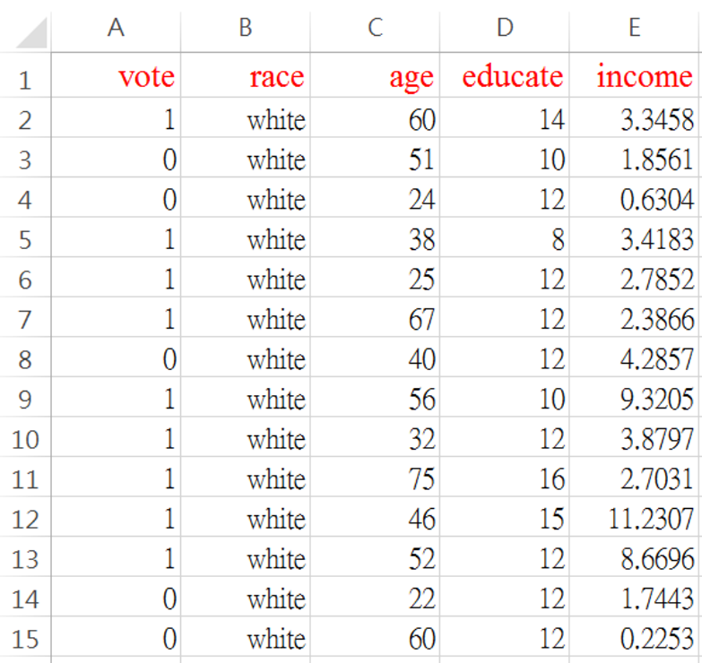
圖 9.1: vote.csv 資料格式
vote =1,有去投票;=0沒有去投票
race =種族別:white=白人;others=其他
age=年齡煙
educate=受教育年數
income=年所得(萬美元)
稱為線性模式的被解釋變數(或Y),數據是連續資料,也就是實數:正、負和小數都可以。和線性模式不同,上面這筆數據的Y是{0, 1}兩個分類別,所以一般也稱為分類問題。這是研究決策科學常遇到的數據, {0, 1} 分別代表解釋變數的二元化行為。研究人員,就會想知道什麼因素決定了特定行為的發生。也因為{0, 1}區間的特性,期望值解讀為機率。
因此,在進入panel data之前,本節簡單解說廣義線性模型(GLM: generalized linear models) 的概念。廣義線性模式應用極多,依照被解釋變數的類別屬性,廣義線性模型可以分為4類:
二元:{0,1},好比 {成功,失敗} 或 {選A,選B}
計數:{50, 100, 199…..},好比在一定時間,餐廳有多少人在用餐
多元:{1,2,3},好比{景氣衰退,景氣反轉,景氣擴張}
有序多元:{1,2,3,4,5},好比{非常不滿意,不滿意,普通,滿意,非常滿意}
二元{0, 1}一般也稱為選擇問題,這是研究決策科學常遇到的數據,{0, 1} 分別代表決策者二分的行為。研究人員會想知道什麼因素決定了特定選擇行為或狀態的發生,例如,有沒有去投票,減重的成功或失敗。也因為{0, 1}區間的特性,期望值解讀為機率。
和線性模式不同,稱為線性模式的被解釋變數(或Y),數據是連續資料,也就是實數:正、負和小數都可以。線性模式不適宜配適Y是 {0, 1}的資料,因為線性配適線是一條直線, 直線的延長會超過{0,1}這個界,如圖9.2:向右方看,要預測高所得的行為機率,就會大於1;往左方看,低所得的機率就會是負的。雖然,線性機率模型預測大體上還可以,但是對於雙尾極端狀況,就會出現預測問題。
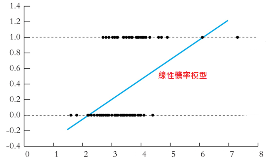
圖 9.2: 線性機率模型
鑑於這種問題,用機率分佈的累積機率密度去配適這樣的資料,應該比較好。也就是圖 9.3。
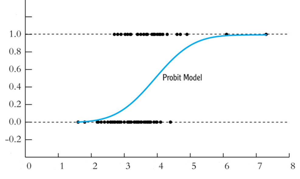
圖 9.3: 機率分佈的累積機率密度
Probit 迴歸利用標準常態分佈的累積機率密度函數 \(\Phi(z)\),估計Y=1 這個事件:也就是,\(z = b_0 + b_1X\)。如下,
\[
Prob(Y=1|X) = \Phi(b_0 + b_1X)
\]
\(\Phi\)是常態分佈的累積密度函數,\(z = b_0 + b_1X\) 稱為 Probit模型的 「z-值」或 「z-指標」。
範例:假設\(b_0 = -2\), \(b_1= 3\), \(X = 0.4\), 所以
\[ Prob(Y=1|X=0.4) = \Phi(-2 + 3 \times 0.4)= \Phi(-0.8) \]
Prob(Y = 1|X=0.4) = 標準常態分佈圖,z = -0.8左邊的面積。如圖 9.4,查表就可以知道機率是多少。當然電腦直接就會幫我們計算。
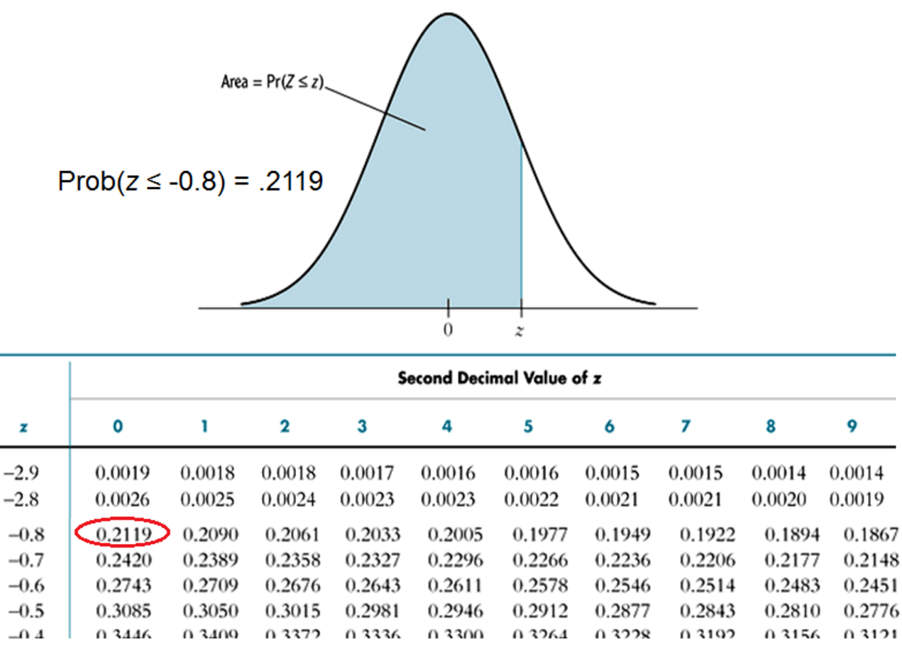
圖 9.4: 標準常態分佈機率
對於二元選擇的Y,Pobit還有一個雙胞胎logit,兩者產生的期望機率大體上是一樣的。Logit函數不連結常態分佈,定義機率生成函數如下:
\[ \tag{9.1} Prob(Y=1|X) =F(b_0+b_1{X})=\frac{1}{1+e^{-(b_0+b_1{X})}} \]
因為Probit 配適一個機率密度函數,在以前計算很慢,所以開發了logit函數。這個時代計算機的演算能力,都沒問題。我們其實不必太嚴格區分兩者。如這裡所介紹的,GLM的估計原理,須要一個連結函數(linking function)來完成,把z和機率函數連結。要連結哪一個機率密度函數,就要看Y的型態是如何。當Y是測量程度,例如,{不滿意,普通,滿意,很滿意} 這樣的行為時,就不是二元選擇(Binary choice),而是多元排序(Ordered Choice),就要編成{0, 1, 2, 3} ,我們就須要用ordered probit/logit;如果Y是「計數」型,好比某時某地的旅遊人數,連結函數就是將這種「隨機變數的條件期望值」和「機率密度函數」連結的函數,一般「計數」型是布阿松函數,所以就是和布阿松函數連結。
因為機率函數是非線性,所以,這一部份也稱為非線性模型。然而,廣義線性的線性,指的是線性連結函數。綜合來說,GLM有三個重要特徵:殘差結構、線性關係、連接函數。
首先,殘差結構,在線性模式往往用常態去處理。但是,這一章的資料則不是常態,被解釋變數的特徵,會出現高度的偏態,峰態,上下界被限制住一定的區間,以及期望值不可為負。所以,殘差結構往往用隨機變數的家族(family)一詞表示。例如,二項式、布阿松、GAMMA等等。
其次,解釋變數和被解釋變數之間,是一個線性關係。
最後,連結函數就是將線性關係產生Y的期望值,與真正的Y觀察值連結起來的函數。基本上,就是一個轉換。線性期望值可能是一個負的值,但是,真正的觀察值卻必須在0和1之間,因此,就需要再轉換一次,讓它更接近Y所描述的現象。這就是連結函數的功能。
式(9.1)的機率函數,一個測量方法是假設log-odds函數: \(log(\frac{p}{1-p})\) ,因此,機率的推導如下:
\[ log(\frac{p}{1-p})=b_0+b_1{X}\\ \frac{p}{1-p}=e^{b_0+b_1X}\\ \frac{1-p}{p}=\frac{1}{e^{b_0+b_1X}}\\ \frac{1}{p}-1=\frac{1}{e^{b_0+b_1X}}\\ \frac{1}{p}=1+\frac{1}{e^{b_0+b_1X}}\\ \frac{1}{p}=\frac{1+e^{b_0+b_1X}}{e^{b_0+b_1X}}\\ p=\frac{e^{b_0+b_1X}}{1+e^{b_0+b_1X}} \]
上式最後可以寫成式(9.1)
\[ \tag{9.2} p=\frac{e^{b_0+b_1X}}{1+e^{b_0+b_1X}}=\frac{1}{1+e^{-(b_0+b_1{X})}} \]
最後,我們必需知道式(9.1)是機率生成函數,不是迴歸方程式,log-odds不是資料。
接下來,我們實做
9.1.1 二元變數之Probit/Logit GLM
範例資料檔沿用 vote.csv。 我們先研究投票和所得與教育水準的關係。 也就說,我們配適GLM於以下三變數方程式
\[
vote=a+b_1{Age} +b_2{Income}+b_3{Education}
\]
我們先繪製投票與否和所得的線性關係。圖 9.5 指出很明顯的線性問題,而且這筆資料的線性配適還蠻嚴重的。
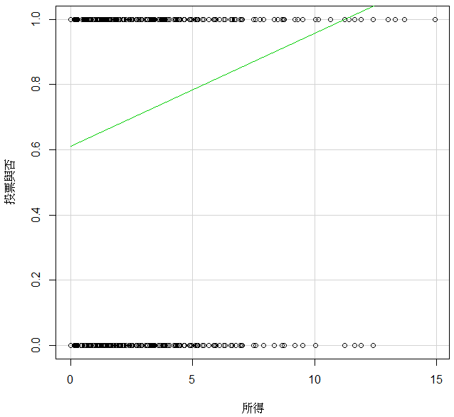
圖 9.5: 投票行為與所得的線性機率模型
R的GLM估計如下。
dat=read.csv("data/vote.csv")
dat$vote=as.factor(dat$vote)
output.logit=glm(vote ~., data=dat,family=binomial(link="logit"))
summary(output.logit)
##
## Call:
## glm(formula = vote ~ ., family = binomial(link = "logit"), data = dat)
##
## Coefficients:
## Estimate Std. Error z value Pr(>|z|)
## (Intercept) -3.034261 0.325959 -9.309 < 2e-16 ***
## racewhite 0.250798 0.146466 1.712 0.0868 .
## age 0.028354 0.003461 8.193 2.54e-16 ***
## educate 0.175634 0.020333 8.638 < 2e-16 ***
## income 0.177112 0.027158 6.521 6.96e-11 ***
## ---
## Signif. codes: 0 '***' 0.001 '**' 0.01 '*' 0.05 '.' 0.1 ' ' 1
##
## (Dispersion parameter for binomial family taken to be 1)
##
## Null deviance: 2266.7 on 1999 degrees of freedom
## Residual deviance: 2024.0 on 1995 degrees of freedom
## AIC: 2034
##
## Number of Fisher Scoring iterations: 5以上,依照三個編號解說:
A. Call 就是執行估計的函數,R的函數是glm(),這樣就一目了然。
B. 係數估計值, 這個結果,只能由符號正負作機率增減的解讀,不能解釋成機率增減幅度。例如,三個參數的p-value都很顯著,所以,以Income為例,我們可以從正相關解釋:所得越高,投票的機率越高。不能 解釋成:所得增加一單位,投票機率增加0.177。
C. 配適檢定。線性模型的配適度,有一個\(R^2\);glm 的配適度使用McFadden \(R^2\),定義如下:
根據上面output下方兩個值,計算得:\(R^2\) = 0.1070993。
另外,估計結果也回傳一個AIC=2034,這個指標越小越好。例如,-200比-150好;但是AIC是比較模型用的,無法用在解讀模型對資料的解釋能力。
接下來,和lm的殘差診斷圖一樣,我們也檢視glm的殘差診斷,如下圖 9.6 。
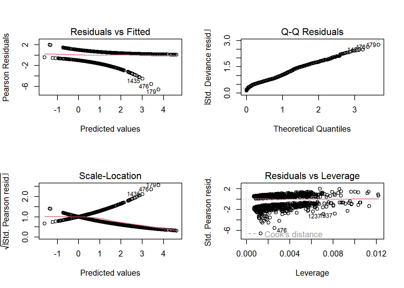
圖 9.6: glm的殘差診斷
〔練習〕估計上述模型,選用Probit看看結果如何。
〔練習〕這筆資料有一個類別變數race:白人與非白人。請增加這個變數,看看種族類別是否與投票行為有關?
再來就是 over-dispersion 和參數變異數修正。理論上,glm 架構的殘差最適表現是卡方分佈。但是,實際上會出現較大的殘差變異,這就稱為over-dispersion。所以,是否須要修正,處理的方法就是先計算dispersion數值,就是殘差平方和除以自由度,也就是模型的變異數。如果dispersion= 1 ,就沒有over-dispersion,也沒有變異數修正問題。如果大於1,就要用這個數值去修正原來的估計結果。分步驟解釋如下:
步驟1。計算dispersion 的經驗值。
估計物件名稱是output.logit,分子是sum(residuals(output.logit)^2),分母自由度是output.logit$df.res,dispersion參數計算公式如下
執行如下
## [1] 1.0145271.014527這個數字很接近1,所以修正的效果應該不太大。
步驟2。如果須要修正,計算完畢後,我們執行下列指令修正標準誤。
如下:
##
## Call:
## glm(formula = vote ~ ., family = binomial(link = "logit"), data = dat)
##
## Coefficients:
##              Estimate Std. Error z value Pr(>|z|)
## (Intercept) -3.034261   0.328318  -9.242  < 2e-16 ***
## racewhite    0.250798   0.147526   1.700   0.0891 .
## age          0.028354   0.003486   8.135 4.13e-16 ***
## educate      0.175634   0.020480   8.576  < 2e-16 ***
## income       0.177112   0.027355   6.475 9.50e-11 ***
## ---
## Signif. codes:  0 '***' 0.001 '**' 0.01 '*' 0.05 '.' 0.1 ' ' 1
##
## (Dispersion parameter for binomial family taken to be 1.014527)
##
##     Null deviance: 2266.7  on 1999  degrees of freedom
## Residual deviance: 2024.0  on 1995  degrees of freedom
## AIC: 2034
##
## Number of Fisher Scoring iterations: 5
對於dispersion值是否須要修正,另外有卡方檢定 dispersion=1.014527,是否顯著大於1。如下:
## [1] 0.3201975這個p-value 接近 0.5,接受無over-dispersion的虛無假設。
另外,套件msme內的函數P__disp(),提供依照pearson方法,如下
## pearson.chi2   dispersion
##  2001.013995     1.003015
pearson.chi2就是依pearson方法計算的殘差平方和,等同以下:
## [1] 2001.014## [1] 1.003015
所以,也不須要使用msme這個套件。最後,顯著性檢定的p-value計算如下:
## [1] 0.4579241
從結果看,兩個p-value 的數值略有差距,結果不變。其實,這個檢定對Disp的數字是很敏感的。讀者可以把Disp手動改成1.2,看看pchisq()計算的p-value變成多少。
基本上,如果我們模型的解釋變數都是正確的,但是出現over-dispersion狀況時,可能的原因是數值刻度沒有適當轉換,或者函數的結構形式不正確。
二元glm的期望值就是機率,R 的計算方法是式(9.2)的logit prob function,我們看R內部計算的預測機率,如下:
##         1         2         3         4         5         6
## 0.8775302 0.6786731 0.5290410 0.5755400 0.6286173 0.8384276
如果把資料集分成樣本內和樣本外,預測時可以用newdata指定資料集,就可以參數套用的指定的新資料,例如:
這個機率可以用來產生二元預測,例如,以0.5為分界點,大於等於0.5的,預測為1,其他為0。
## 1 2 3 4 5 6
## 1 1 1 1 1 1
這個預測結果,可以和真實資料製作混淆矩陣來評估預測能力,不在此說。
最後,我們用人工方法,依照式(9.2)整理資料,計算預測機率
dat.tmp=dat
dat.tmp$race=as.integer(as.factor(dat$race))-1
dat.tmp=cbind(1,dat.tmp[,-1])
colnames(dat.tmp)=names(output.logit$coef)
score.logit=as.matrix(dat.tmp) %*% as.matrix(output.logit$coef)
prob.logit.formula=c(exp(score.logit)/(1+exp(score.logit))) #用式(9.2)計算機率
head(prob.logit.formula)
## [1] 0.8775302 0.6786731 0.5290410 0.5755400 0.6286173 0.8384276可以用以下方式檢測,可知兩個方法完全相等。
## [1] TRUE最後,如果使用”probit”,如下,就是配適常態機率密度,而不是(9.2),我們可以用類似方法檢驗。
output.probit=glm(vote ~., data=dat,family=binomial(link="probit"))
prob.probit.pred=predict(output.probit,type="response")
head(prob.probit.pred)
## 1 2 3 4 5 6
## 0.8793837 0.6784155 0.5430547 0.5757100 0.6301197 0.8380967score.probit=as.matrix(dat.tmp) %*% as.matrix(output.probit$coef)
prob.probit.pnorm=pnorm(score.probit) #用常態分佈計算機率
head(prob.probit.pnorm)## [,1]
## [1,] 0.8793837
## [2,] 0.6784155
## [3,] 0.5430547
## [4,] 0.5757100
## [5,] 0.6301197
## [6,] 0.8380967可以用以下方式檢測是否相等
## [1] TRUE9.1.2 計數型變數之布阿松迴歸– Poisson GLM
什麼是布阿松迴歸?布阿松迴歸適合用於對結果為計數的事件或列聯表進行建模的統計方法。或者,更具體地說,計數數據:具有非負整數值的離散數據,用於計數某些內容,例如在給定時間範圍內事件發生的次數或在雜貨店排隊的人數。計數數據也可以表示為速率數據,因為事件在時間範圍內發生的次數可以表示為原始計數(即“一天中,步行30公里”)或平均速率(“我們以平均每小時1.25公里的速度步行”)。計數型的被解釋變數在現實生活中還不少,例如,特定時間的:政治倒閣次數,車禍次數,排隊結帳的人數,以及社群媒體按讚人數。
布阿松迴歸允許我們確定哪些解釋變數X對給定的被解釋變數Y(計數或速率)有影響,從而幫助我們分析計數數據和速率數據。例如,銀行可以應用布阿松迴歸來更好地瞭解和預測排隊等待服務的人數。
如前一節的二元分佈須要logistic或常態分佈的機率函數為MLE的基礎,布阿松迴歸須要布阿松分佈。布阿松分佈是一種以法國數學家Siméon Denis Poisson命名的統計理論。它對事件或事件y 在特定時間範圍內發生的概率進行建模,假設 y 的發生不受 y 的先前出現時間的影響。機率密度函數定義如下:
\[ p(y)=\frac{{\lambda}^{y}{e^{-{\lambda}}}}{y!} \]
在這裡,\(\lambda\) 就是期望值,也就是說:\(\lambda=\mu\),也就是是每單位暴露事件可能發生的平均次數。暴露可以是時間、空間、人口規模、距離或面積,但通常是時間,用 t 表示。如果未給出曝光值,則假定它等於 1。布阿松隨機變數的一個性質是期望值和變異數都是\(\lambda\),我們可以通過為不同的 \(\lambda\) 值,創建機率分布圖來視覺化這一個性質,有興趣的讀者,可以透過機率教科書,試著做做看。
布阿松迴歸模型是一種廣義線性模型 (GLM),用於對計數數據和列聯表進行建模。輸出 Y(計數)是遵循布阿松分佈的值。它假設期望值(平均值)的對數,可以通過一些未知參數建模為線性形式。
注意:在統計學中,列聯表(示例)是取決於多個變數的頻率矩陣。
為了將非線性關係轉換為線性形式,使用了連結函數,該函數是泊松回歸的對數。因此,布阿松迴歸模型也稱為對數線性(log-linear)模型。布阿松迴歸模型的一般數學形式為:
\[ log(y)=a+b_{1}x_{1}+...+b_{k}x_{k}+\epsilon \] 故,
\[ y=e^{a+b_{1}x_{1}+...+b_{k}x_{k}+\epsilon} \] 用矩陣表示條件期望值,\(E[y|X]=e^{\beta X}\),因為分佈函數的性質:\(E[y|X]=\lambda\),我們可以將之代入機率密度函數,如下:
\[ p(y|x;\beta)=\frac{{(E[y|X])}^{y}{e^{-{(E[y|X])}}}}{y!}=\frac{e^{y{\beta}X}{e^{-{(\beta}X)}}}{y!} \]
承上,就可以用MLE求解概似函數。最大概似函數估計\(\beta\)的核心想法是,去找到能使得基於當前觀測值的聯合概率儘可能達到最大的\(\beta\)。(可理解為:變量的取值當前觀測值,與取值為其他任何數值相比,是發生機率最高的事件)。既然目標是尋找到最優的\(\beta\),可以先將上式的等號左邊簡單表達為關於\(\beta\)的表達式。這些技術細節,有興趣的讀者可以去看相關書籍,本書大致簡介到這邊。接下來實做:
本節的範例檔用 countStrikes.csv,這筆資料欲研究罷工次數的影響因素。這筆資料表的形式如下。
##   NUMB_strike FEB    IP
## 1           5   0 1.517
## 2           4   1 0.997
## 3           6   0 0.117
## 4          16   0 0.473
## 5           5   0 1.277
## 6           8   0 1.138
變數解釋如下:
NUMB_strike: 罷工次數
FEB: =1, 發生在二月;0=其他月份
IP:以工業生產指數變動率計算的經濟成長,%
我們的被解釋變數是Numb_strike,估計這種隨機變數,機率分佈模型是布阿松。連結函數只是轉換成機率時用的函數,如果用線性,數值結果會有些許差異,但是增減方向不變。說明範例如下:
發生罷工次數的時間,二月比其他月份的平均次數要少;經濟成長率較高,平均罷工次數也較高。
##
## Call:
## glm(formula = NUMB_strike ~ ., family = poisson(link = "log"),
##     data = dat.pois)
##
## Coefficients:
##              Estimate Std. Error z value Pr(>|z|)
## (Intercept)  1.725630   0.043656  39.528  < 2e-16 ***
## FEB         -0.377407   0.174520  -2.163 0.030577 *
## IP           0.027753   0.008191   3.388 0.000703 ***
## ---
## Signif. codes:  0 '***' 0.001 '**' 0.01 '*' 0.05 '.' 0.1 ' ' 1
##
## (Dispersion parameter for poisson family taken to be 1)
##
##     Null deviance: 241.71  on 102  degrees of freedom
## Residual deviance: 224.86  on 100  degrees of freedom
## AIC: 575.09
##
## Number of Fisher Scoring iterations: 5
接下來,和二元glm一樣,我們也檢視glm-poisson的殘差診斷,如下圖 9.7 。
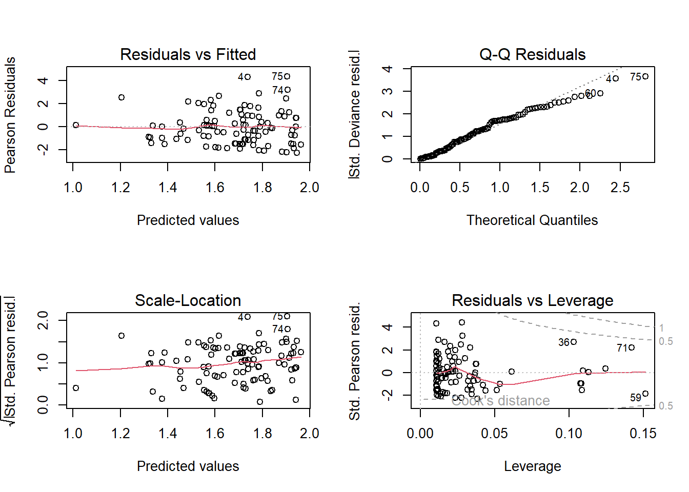
圖 9.7: glm-poisson的殘差診斷
剩下的實做問題,和二元差不多,我們設計成練習問題,讓有趣的讀者練習。
〔練習〕用fitted() 比較三個連結函數預測的平均罷工次數,差異如何。
〔練習〕請計算Over-dispersion,並修正原估計結果。
〔練習〕解讀圖 9.7的意義
9.1.3 多元選擇 GLM— Multinomial Probit/Logit
二元選擇的問題,行為者的選擇是二選一。一個更普遍的情況是行為者是從多個選項中選擇一個,如下健康保險資料mlogit.csv的欄位變數。
##   patient_ID    insure age    sex white ppd0 ppd1 ppd2 ppd site noinsur0
## 1       3292 Indemnity  74 Female   Yes    0    0    0   0    2        0
## 2       3685   Prepaid  28 Female   Yes    1    1    1   1    2       NA
## 3       5097 Indemnity  38 Female   Yes    0    0    0   0    1        0
## 4       6369   Prepaid  24 Female    No    1    1    1   1    3       NA
## 5       9194   Prepaid  30 Female   Yes    1    1    1   1    2       NA
## 6      11492   Prepaid  39 Female   Yes    1    1    1   1    2       NA
##   noinsur1 noinsur2
## 1        0        0
## 2       NA       NA
## 3        0        0
## 4       NA       NA
## 5       NA       NA
## 6       NA       NA
Insure 是我們的被解釋變數,有三項:
indemnity: 保險損害賠償。
prepaid: 預付計畫,如HMO(health maintenance organization 維護健康組織)的計畫。預付一筆費用,就可以無限使用。
Uninsure: 沒有保險
其他欄位代表:
Sex: 性別
White: 是否為白人
ppd0: prepaid at baseline
ppd1: prepaid at year 1
ppd2: prepaid at year 2
這筆資料用來研究病人對於方案的選擇和人口因素的關連。類似資料研究的問題,教育方面有大學生畢業後的選擇:碩士、就業、留學。載入資料後,以insure為被解釋變數,解釋變數配適年齡(age)、性別(sex)和種族(White)三個變數。
output.mlogit=nnet::multinom(insure~age+sex+white, data=dat.mlogit,maxit=1000,trace=FALSE)
summary(output.mlogit)
## Call:
## nnet::multinom(formula = insure ~ age + sex + white, data = dat.mlogit,
## maxit = 1000, trace = FALSE)
##
## Coefficients:
## (Intercept) age sexMale whiteYes
## Prepaid 0.8874833 -0.011179932 0.5745660 -0.7312471
## Uninsure -1.3739253 -0.005927721 0.5109524 -0.4335456
##
## Std. Errors:
## (Intercept) age sexMale whiteYes
## Prepaid 0.3400588 0.006101655 0.2005740 0.2189813
## Uninsure 0.6372029 0.011433969 0.3640691 0.4106268
##
## Residual Deviance: 1091.184
## AIC: 1107.184估計結果中會將被解釋變數的3個類別視為base,R裡面是自動依字母排序,排在前面的就是indemnity。base的項目,就是和其他兩個比較的。所以,這結果的解讀,必須小心。下半部估計結果,R對結果的輸出,是依照估計項目去分2部份:Coefficients(係數)和Std.
以係數為例的解讀如下:
第1. 截距代表了三個變數的觀察值是0時的機率,可執行兩行語法計算
cc=c(0, 0.8874, -1.3739)
exp(cc)/sum(exp(cc))
## [1] 0.27159710 0.65965682 0.06874608
三者機率差異很大,意思是說:當三個變數的觀察值是0時(女性且非白人),個人選擇indemnity的機率是0.2715971,選擇prepaid的機率是0.65965682,選擇不保險的機率是0.06874608。
第2. 斜率代表了log-odds機率,測量了1個人從選擇baseline(=indemnity),過渡到選擇prepaid或選擇uninsured的機率。例如,age斜率是-0.011和-0.0059
cc=c(0, -0.0112, -0.0059)
exp(cc)/sum(exp(cc))
## [1] 0.3352353 0.3315016 0.3332632
三者機率類似,意思是說:年齡增加1歲,從「選擇baseline」(=indemnity)」,過渡到「選擇prepaid」的機率是0.3315016,過渡到「選擇 uninsured」的機率是0.3332632。
其餘關於over-dispersion計算與問題,皆與上同。有趣讀者可以試試看。
9.2 Panel Data的類別資料– panel GLM
9.2.1 原理淺說
panel GLM 的理論問題說難也很難,說簡單也很簡單。基於 第二章起的panel data和前一節類別資料GLM的理解,panel GLM似乎也就沒那麼難。我想先淺談一些理論問題。
在線性模型時,固定效果的概念就是被解釋變數的de-mean,移除平均數。如果Y是連續的,這個LSDV的動作沒有問題,但是Y是二元類別數據時,這個動作就沒有意義了。何況,更多的二元資料是用文字表示的因子,例如,{成功,失敗}或{No, Yes},這樣,就不能用LSDV去計算固定效果,因此,基本的情況就是使用隨機效果或pooling方法。不少商業經濟計量軟體是採用pooling來處理二元panel data,例如,Eviews。
然後,理論上, Chamberlain (1980) 指出通過條件概似函數(conditional likelihood),搜索最小的充分統計量(sufficient statistic), Chamberlain (1980) 證明,對於個別效果,\(y_{it}\)的總和是一個最小的充分統計量。 因此,最大化條件概似函數,
下面的函數可以生成conditional logit的參數估計式,且避免了擾攘參數的問題:
\[ {{L}_{c}}=\prod\limits_{\text{i}=\text{1}}^{\text{N}}{\text{Prob}\left( {{\text{y}}_{\text{i1}}}\text{,}{{\text{y}}_{\text{i2}}}\text{,}\cdots {{\text{y}}_{\text{iT}}}|\sum\limits_{t=1}^{T}{{{y}_{it}}} \right)} \]
並且,根據充分統計的定義,在特定統計量之下的分佈,將不依賴於個別效果 \(\mu_{i}\)。也就是說,藉著conditioning on \(y_{it}\) 可以移除個別效果的影響(incidental parameter problem)。這個意思就是說,在「非嚴格的實證需求」意義下,二元類別變數涉及panel data時,我們或許可以不必顧慮固定效果和隨效果的選擇問題,也就是Hausman test。
所謂「非嚴格的實證需求」這個實務思路,類似線性panel data時,如果解釋變數出現類別時,例如,性別,工作類別,居住地區等等;而且我們研究的目的事要知道些類別解釋變數的影響,就無法使用固定效果,因為LSDV (or de-mean) 會將之全數移除。因為研究目的需要,只能使用隨機效果才能檢視這些變數。
經濟計量方法關於二元類別變數的討論多半是相當理論,例如,Chamberlain (2010) 在的論文。如果涉及動態,請參考 Honoré and Kyriazidou (2000) ,都是 Econometrica 的論文,相當艱澀。
9.2.2 R 實做– 二元資料
我們使用的套件是 plm 的姊妹作品 pglm,資料是內建的 UnionWage,如果是由外部載入,必需宣告panel data.frame才能繼續使用。我們先介紹一個和內建的 UnionWage 完全一樣的 UnionWage.csv,之後,都使用內建資料。
先 library(pglm) 載入套件
UnionWage.tmp=read.csv("data/UnionWage.csv")
UnionWage=pdata.frame(UnionWage.tmp,index = c("id", "year"))
head(UnionWage,10)
## id year exper health hours married rural school union wage
## 13-1980 13 1980 1 no 2672 0 no 14 no 1.1975402
## 13-1981 13 1981 2 no 2320 0 no 14 yes 1.8530600
## 13-1982 13 1982 3 no 2940 0 no 14 no 1.3444617
## 13-1983 13 1983 4 no 2960 0 no 14 no 1.4332133
## 13-1984 13 1984 5 no 3071 0 no 14 no 1.5681251
## 13-1985 13 1985 6 no 2864 0 no 14 no 1.6998909
## 13-1986 13 1986 7 no 2994 0 no 14 no -0.7202626
## 13-1987 13 1987 8 no 2640 0 no 14 no 1.6691879
## 17-1980 17 1980 4 no 2484 0 no 13 no 1.6759624
## 17-1981 17 1981 5 no 2804 0 no 13 no 1.5183982
## sector occ com region
## 13-1980 businessrepair service white NorthEast
## 13-1981 personalservice service white NorthEast
## 13-1982 businessrepair service white NorthEast
## 13-1983 businessrepair service white NorthEast
## 13-1984 personalservice craftfor white NorthEast
## 13-1985 businessrepair manoffpro white NorthEast
## 13-1986 businessrepair manoffpro white NorthEast
## 13-1987 businessrepair manoffpro white NorthEast
## 17-1980 trade manoffpro white NorthEast
## 17-1981 trade manoffpro white NorthEast
變數說明:
id = the cross-section individual index
year= the time index
exper= the experience, computed as age - 6 - schooling
health= does the individual has health disability ?
hours= the number of hours worked
married= is the individual married ?
rural= does the individual lives in a rural area ?
school= years of schooling
union= does the wage is set by collective bargaining
wage= hourly wage in US dollars
sector= one of agricultural, mining, construction, trade, transportation, finance, businessrepair, personalservice, entertainment, manufacturing, pro.rel.service, pub.admin
occ = one of proftech, manoffpro, sales, clerical, craftfor, operative, laborfarm, farmlabor, service
com = one of black, hisp and other
region= the region, one of NorthEast, NothernCentral, South and other
首先,使用pooling 資料結構估計二元資料
pglm.pooling <- pglm(union ~ wage + exper + rural, data=UnionWage, family = binomial(‘logit’),
model = “pooling”, method = “bfgs”, print.level = 3, R = 5)
其次,檢視估計係數。
##                Estimate Std. error     t value      Pr(> t)
## (Intercept) -2.28446068 0.15068399 -15.1606066 6.447112e-52
## wage         0.72411012 0.07588823   9.5417977 1.403775e-21
## exper       -0.01410725 0.01308915  -1.0777819 2.811311e-01
## ruralyes     0.08068956 0.08999071   0.8966432 3.699093e-01
pooling方法沒有任何橫斷面處理,就是一般的glm。我們可以檢視glm的結果,如下:
datz=UnionWage.tmp[,-c(1,2)]
datz$union=as.integer(as.factor(datz$union))-1
summary(glm(union ~ wage + exper + rural, data=datz, family = binomial('logit')))
##
## Call:
## glm(formula = union ~ wage + exper + rural, family = binomial("logit"),
## data = datz)
##
## Coefficients:
## Estimate Std. Error z value Pr(>|z|)
## (Intercept) -2.28446 0.15068 -15.161 <2e-16 ***
## wage 0.72411 0.07589 9.542 <2e-16 ***
## exper -0.01411 0.01309 -1.078 0.281
## ruralyes 0.08069 0.08999 0.897 0.370
## ---
## Signif. codes: 0 '***' 0.001 '**' 0.01 '*' 0.05 '.' 0.1 ' ' 1
##
## (Dispersion parameter for binomial family taken to be 1)
##
## Null deviance: 4845.6 on 4359 degrees of freedom
## Residual deviance: 4746.3 on 4356 degrees of freedom
## AIC: 4754.3
##
## Number of Fisher Scoring iterations: 4我們可以發現兩者完全一樣。也就是說,如果您想使用pooling 估計類別panel data,那個用glm這個方法更好,因為所有的檢測都可以做,包括用predict()執行機率預測。在套件pglm,只提供了估計。
再來,使用random effect 設定估計二元資料
pglm.RE <- pglm(union ~ wage + exper + rural, data=UnionWage, family = binomial(‘logit’), model = “random”, method = “nr”, print.level = 3, R = 5)
其次,檢視估計係數。
##                Estimate Std. error     t value       Pr(> t)
## (Intercept) -3.18669099 0.25818524 -12.3426537  5.336747e-35
## wage         0.74243612 0.14032956   5.2906611  1.218750e-07
## exper       -0.04532529 0.02194934  -2.0649957  3.892341e-02
## ruralyes     0.07931936 0.21513642   0.3686933  7.123563e-01
## sigma        2.32635513 0.08005005  29.0612591 1.109018e-185
隨機效果多了一個底列的變異數估計,其餘參數和pooling 的結果都很接近。pglm沒有提供預測函數,也沒有dispersion值;所以,用pglm只能估計,其餘如預測,都必需自己來。這也是為什麼在本章前面,要詳細解釋標準glm的機率計算方法。
9.2.3 some count data models
接下來,我們用內建的專利資料,執行布阿松的panel GLM。資料如下:
##   cusip year ardssic scisect  capital72 sumpat         rd patents
## 1   800 1970      15      no 438.605335    354  2.7097056      30
## 2  1030 1970      14     yes   7.206043     13  0.6324526       3
## 3  2824 1970       4     yes 284.004476    493 29.6819762      48
## 4  4644 1970      13      no   1.981333      2  1.7218512       1
## 5  7842 1970      16      no   7.880017     12  1.4845475       2
## 6 10202 1970       3      no 396.533291    393  7.8366387      32
變數說明:
cusip= compustat’s identifying number for the firm
year= year
ardssic= a two-digit code for the applied R&D industrial classification
scisect= is the firm in the scientific sector ?
capital72= book value of capital in 1972
sumpat= the sum of patents applied for between 1972-1979
rd = R&D spending during the year (in 1972 dollars)
patents= the number of patents applied for during the year that were eventually granted
很明顯地,被解釋變數是專利數patents。計數型資料,固定效果,隨機效果皆可
首先,使用固定效果。布阿松的family有兩個宣告可以用:“negbin” 和 “poisson”。
output.pois.FE <- pglm(patents ~ lag(log(rd), 0:5) + scisect + log(capital72) + factor(year), PatentsRDUS,family = negbin, model = “within”, print.level = 3, method = “nr”,
index = c(‘cusip’, ‘year’))
檢視係數。
##                        Estimate Std. error     t value      Pr(> t)
## (Intercept)         1.661391906 0.34355211  4.83592411 1.325285e-06
## lag(log(rd), 0:5)0  0.272678998 0.07078382  3.85227868 1.170237e-04
## lag(log(rd), 0:5)1 -0.097886613 0.07679202 -1.27469765 2.024163e-01
## lag(log(rd), 0:5)2  0.032076216 0.07086391  0.45264529 6.508042e-01
## lag(log(rd), 0:5)3 -0.020392326 0.06577085 -0.31005112 7.565221e-01
## lag(log(rd), 0:5)4  0.016221420 0.06288501  0.25795369 7.964426e-01
## lag(log(rd), 0:5)5 -0.009727993 0.05328640 -0.18256051 8.551429e-01
## scisectyes          0.017639777 0.19807352  0.08905672 9.290368e-01
## log(capital72)      0.207148837 0.07796793  2.65684680 7.887528e-03
## factor(year)1976   -0.038392668 0.02447217 -1.56882972 1.166876e-01
## factor(year)1977   -0.039940327 0.02522746 -1.58320824 1.133740e-01
## factor(year)1978   -0.144327802 0.02645968 -5.45463173 4.907444e-08
## factor(year)1979   -0.195751826 0.02716372 -7.20637068 5.746284e-13
其次,使用pooling估計。
output.pois.pool <- pglm(patents ~ lag(log(rd), 0:5) + scisect + log(capital72) + factor(year), PatentsRDUS, family = “poisson”, model = “pooling”, index = c(“cusip”, “year”), print.level = 0, method=“nr”)
檢視係數。
##                        Estimate  Std. error     t value      Pr(> t)
## (Intercept)         0.809909894 0.021188565  38.2239147 0.000000e+00
## lag(log(rd), 0:5)0  0.134524577 0.030718260   4.3793033 1.190594e-05
## lag(log(rd), 0:5)1 -0.052944368 0.042797205  -1.2370987 2.160504e-01
## lag(log(rd), 0:5)2  0.008229465 0.039784462   0.2068512 8.361261e-01
## lag(log(rd), 0:5)3  0.066096918 0.036968573   1.7879218 7.378862e-02
## lag(log(rd), 0:5)4  0.090181342 0.033336156   2.7052112 6.826098e-03
## lag(log(rd), 0:5)5  0.239538388 0.022459775  10.6652175 1.480523e-26
## scisectyes          0.454309575 0.009242341  49.1552483 0.000000e+00
## log(capital72)      0.252862548 0.004414258  57.2831414 0.000000e+00
## factor(year)1976   -0.043515208 0.013120942  -3.3164698 9.116243e-04
## factor(year)1977   -0.052441295 0.013287569  -3.9466433 7.925451e-05
## factor(year)1978   -0.170242204 0.013529768 -12.5827878 2.625965e-36
## factor(year)1979   -0.201878694 0.013533502 -14.9169594 2.556605e-50
最後,使用隨機效果估計。
output.pois.RE <- pglm(patents ~ lag(log(rd), 0:5) + scisect + log(capital72) + factor(year), PatentsRDUS, family = poisson, model = “random”, index = c(“cusip”, “year”),
print.level = 0, method=“nr”)
檢視係數。
##                       Estimate Std. error     t value      Pr(> t)
## (Intercept)         0.41078760 0.14674431   2.7993425 5.120679e-03
## lag(log(rd), 0:5)0  0.40345381 0.04350220   9.2743314 1.787365e-20
## lag(log(rd), 0:5)1 -0.04617658 0.04822236  -0.9575761 3.382765e-01
## lag(log(rd), 0:5)2  0.10792359 0.04471154   2.4137749 1.578822e-02
## lag(log(rd), 0:5)3  0.02977315 0.04132353   0.7204890 4.712239e-01
## lag(log(rd), 0:5)4  0.01069573 0.03770738   0.2836508 7.766780e-01
## lag(log(rd), 0:5)5  0.04061105 0.03157378   1.2862271 1.983638e-01
## scisectyes          0.25700007 0.11227165   2.2890914 2.207404e-02
## log(capital72)      0.29169335 0.03933681   7.4152772 1.213707e-13
## factor(year)1976   -0.04496242 0.01312912  -3.4246327 6.156312e-04
## factor(year)1977   -0.04838634 0.01340178  -3.6104417 3.056760e-04
## factor(year)1978   -0.17416192 0.01397018 -12.4666875 1.134445e-35
## factor(year)1979   -0.22589767 0.01466453 -15.4043572 1.530031e-53
## sigma               1.16968955 0.09471381  12.3497258 4.887775e-35
雖然,pglm是glm的姊妹作品,但是多數plm的檢定,都不適用。畢竟很多 lm 可以作的檢定,在 glm 也不能做,反之亦然;panel data的狀況也是這樣。但是,透過混淆矩陣,可以分析比較模型的好壞,和分類演算法完全一樣。這一部份,晚一點再補進來。
9.3 從多層次模型的角度看panel GLM
本書第6章談序列相關修正問題時,曾介紹過使用MLM架構來處理。從資料結構的角度,panel data只是多層次資料(multilevel data)的一個特例。其實 multilevel data 比 panel data 更為一般化,也可處理nested panel,例如 \(y_{ijk,t}\) 這樣的層次結構。除非讀者須要執著在計量經濟學的胡同做研究,不然多層次模型(multilevel linear model,MLM)會是更好的選擇,給予我們更為彈性的架構來分析資料。
我在這裡解說panel glm 的一些問題,也利用這節叮嚀研究人員如果遇到 categorical panel data,首選是MLM的 lme4,而不是 pglm。原因在於pglm 有一些套件功能性缺失,讓我們利用預測評估多個模型相當困難。
基本上,在類別資料時,如果用pooling方式,則 glm就可以完善處理;其餘,如固定效果,隨機效果,乃至 two-way 設定,MLM都可以處理。這一節,我們用混淆矩陣來說明預測問題。其餘模型,讀者熟悉語法後,自然可以在MLM架構下處理。
9.3.1 預測
第1步:我們取用前面 UnionWage 二元資料與 pglm 的隨機效果物件 pglm.RE,重看一次係數。
##                Estimate Std. error     t value       Pr(> t)
## (Intercept) -3.18669099 0.25818524 -12.3426537  5.336747e-35
## wage         0.74243612 0.14032956   5.2906611  1.218750e-07
## exper       -0.04532529 0.02194934  -2.0649957  3.892341e-02
## ruralyes     0.07931936 0.21513642   0.3686933  7.123563e-01
## sigma        2.32635513 0.08005005  29.0612591 1.109018e-185
第2步:預測。因為pglm沒有提供預測函數,然而在panel 演算中,有許多處理必需還原,例如隨機效果值必需還原加回去才可以計算期望值。這些需求,plm都有,但是pglm都沒有;所以,如果利用標準glm算法,會出現計算失敗的結果,如下展示:
data.pglm.re=UnionWage
data.pglm.re$union=as.integer(as.factor(UnionWage$union))-1
data.pglm.re$rural=as.integer(as.factor(UnionWage$rural))-1
data.pglm.re0=cbind(1,data.pglm.re[,colnames(pglm.RE$model)[-1]])
score.pglm.re=as.matrix(data.pglm.re0)%*% as.matrix(coef(pglm.RE)[1:4])
prob.pglm.re=c(exp(score.pglm.re)/(1+exp(score.pglm.re)))
prediction.pglm.re=ifelse(prob.pglm.re>=0.5,1,0)
table(prediction.pglm.re)
## prediction.pglm.re
## 0
## 4360我們利用table()發現所有的預測都是0,這樣就沒有用了。畢竟我們的資料有3296個0(no),1064個1(yes)。這不是pglm計算錯,而是回傳物件太少,讓我們必需花很大精神還原。接下來,我們看看MLM是否就沒有這問題。
首先,估計MLM隨機效果模型,如下:(1|id)宣告個別效果id以隨機效果方式處理。此處和第6章不同的地方在於使用了glmer()函數,而不是lmer()函數。
## 載入需要的套件:Matrixdat.mlm=UnionWage.tmp
dat.mlm$union=as.integer(as.factor(UnionWage.tmp$union))-1
mlm.RE <- glmer(union ~ (1|id) + wage + exper + rural , data=dat.mlm, family =binomial(link="logit"))估計完後,我們取出如下係數
##                Estimate Std. Error     z value     Pr(>|z|)
## (Intercept) -3.56146283 0.31553439 -11.2870830 1.519977e-29
## wage         0.84099466 0.15672045   5.3662087 8.040888e-08
## exper       -0.06689668 0.02346379  -2.8510600 4.357375e-03
## ruralyes     0.12337240 0.23604472   0.5226654 6.012071e-01
MLM係數和pglm係數,只有些微差距,因此,MLM的預測結果,應該很接近。我們先看MLM的預測,如下語法:
prob.mlm.re=predict(mlm.RE,type="response")
prediction.mlm.re=ifelse(prob.mlm.re>=0.5,1,0)
table(prediction.mlm.re)
## prediction.mlm.re
## 0 1
## 3460 900
我們發現預測還不錯,但是正確程度與否要和原始值配對。類別資料採用混淆矩陣,最簡單的就是套件caret的confusionMatrix函數,如下
CF.mlm.re=table(prediction=as.numeric(prediction.mlm.re),actual=dat.mlm$union)
caret::confusionMatrix(CF.mlm.re)
## Confusion Matrix and Statistics
##
## actual
## prediction 0 1
## 0 3141 319
## 1 155 745
##
## Accuracy : 0.8913
## 95% CI : (0.8817, 0.9004)
## No Information Rate : 0.756
## P-Value [Acc > NIR] : < 2.2e-16
##
## Kappa : 0.6891
##
## Mcnemar's Test P-Value : 7.055e-14
##
## Sensitivity : 0.9530
## Specificity : 0.7002
## Pos Pred Value : 0.9078
## Neg Pred Value : 0.8278
## Prevalence : 0.7560
## Detection Rate : 0.7204
## Detection Prevalence : 0.7936
## Balanced Accuracy : 0.8266
##
## 'Positive' Class : 0
## 若以0為positive,根據混淆矩陣的績效計算,我們發現正確度(Accuracy)達到0.89,精確度(precision 或 Pos Pred Value)達到0.9078,召回率(Recall 或Neg Pred Value)達到0.8278;校正觀察與機率符合度的 kappa 則是 0.6891,算是相當好(kappa>0.4可以算是有參考價值的結果)。
如果研究者只須要係數,那麼 pglm 完全沒問題。如果須要處理訓練集和測試集的問題,則樣本外預測就會是一個重要架構,pglm目前是完全無法妥善處理。
9.3.2 序列相關修正
panel data的類別資料,因為有時間序列,所以,不可避免的會出現序列相關問題,因此,如第6章,序列相關的影響會導致估計解果出現bias。因此,就須要校正序列相關的影響。這類問題,較容易出現在布阿松,例如,之前使用的專利。例如,一個產業的專利,會和前一年有關。pglm如果添加落後期來處理序列相關,會導致動態問題,在類別資料很不容易處理。本節介紹在布阿松分佈時,序列相關校正的作法。
R套件有數個處理AR(1)的套件,主要有兩個發佈在CRAN: glmmPQR 和 glmmTMB。glmmPQR 是MASS的函數,glmmTMB則完全屬於glmmTMB套件。很可惜地,兩個套件的結果差距很大,這一點,我要謝謝UT Austin的林澤民教授,沒有他指出,我都不知道有這麼大差異。所以,我們先用simulation看看兩個套件,哪一個才是我們應該用的。
9.3.2.1 poisson 型
第1步。我們先用模擬數據產生具AR(1)的布阿松數據,如下:
sim.AR1 <- function(ar1=0.7,sdGroup=2,sdres=1,
                    nperGroup=50,nGroup=200,seed=NULL,
                    linkinv="identity",simfun="identity",
                    dist=c("mvrnorm","rmvt")) {

  if (!is.null(seed)) set.seed(seed)
  cmat <- sdres*ar1^abs(outer(0:(nperGroup-1),0:(nperGroup-1),"-"))

  if (dist=="rmvt") {
    errs <- LaplacesDemon::rmvt(n=nGroup, mu=runif(nperGroup), S=cmat, df=Inf)
    } else {
    errs <- MASS::mvrnorm(nGroup,mu=runif(nperGroup),Sigma=cmat)
    }

  ranef <- rnorm(nGroup,mean=sample(0:10,1),sd=sdGroup)
  df <- data.frame(ID=rep(1:nGroup,each=nperGroup))
  eta <- ranef[as.numeric(df$ID)] + c(t(errs)) ## unpack errors by row
  mu <- linkinv(eta)
  df$y <- simfun(mu)
  df$year <- factor(rep(1:nperGroup,nGroup))
  return(df)
}
sim.AR1是模擬程式,允許多變量的常態分佈和student t分佈。
第2步。DGP,令AR(1)係數為0.8,t=20, N=250,先用常態分佈。 因為我們要比較序列相關的校正,所以DGP就不生成解釋變數。
sim.pois <- sim.AR1(ar1=0.8,nperGroup=20,nGroup=250,dist=c("mvrnorm","rmvt")[1],
              linkinv=exp,simfun=function(x) rpois(length(x),lambda=x))
out.pglm.RE=plm::plm(y~lag(y,1),data=sim.pois, model = "random",index="ID")
coef(summary(out.pglm.RE))
## Estimate Std. Error z-value Pr(>|z|)
## (Intercept) 90.585661 13.365664031 6.777491 1.222812e-11
## lag(y, 1) 0.738531 0.009403339 78.539228 0.000000e+00## Estimate Std. Error t-value Pr(>|t|)
## lag(y, 1) 0.4660618 0.01270094 36.69505 4.059389e-258
我們發現這筆資料套用 plm 檢視線性一階自我相關,隨機效果的話,可以確認AR(1)較接近0.8,bias 較低;固定效果時,AR(1)係數=0.378,bias較高。這樣也給我們提供一種檢視資料序列相關程度的方法
第3步。配適MASS::glmmPQR
out.PQL=MASS::glmmPQL(y ~ 1,random= ~1|ID, data=sim.pois,family="poisson",
                      correlation=nlme:::Initialize(nlme:::corAR1(0.5, form = ~ 1|ID), sim.pois),
                      verbose=FALSE, niter = 150)
print(out.PQL)
## Linear mixed-effects model fit by maximum likelihood
## Data: sim.pois
## Log-likelihood: NA
## Fixed: y ~ 1
## (Intercept)
## 4.595846
##
## Random effects:
## Formula: ~1 | ID
## (Intercept) Residual
## StdDev: 1.47934 18.44052
##
## Correlation Structure: AR(1)
## Formula: ~1 | ID
## Parameter estimate(s):
## Phi
## 0.5287646
## Variance function:
## Structure: fixed weights
## Formula: ~invwt
## Number of Observations: 5000
## Number of Groups: 250我們發現估出來的AR(1)係數 \(\phi \sim 0.5\),和模擬假設的0.8差距甚遠, 接下來,我們看殘差的序列相關降低多少,如下:
dat.PQL=data.frame(id=sim.pois$ID,year=sim.pois$year, e=residuals(out.PQL))
plm::plm(e~lag(e,1),data=dat.PQL,index="id", method="within") #Residuals ar(1) check
##
## Model Formula: e ~ lag(e, 1)
##
## Coefficients:
## lag(e, 1)
## 0.43012降低約不到一半,0.366。
第4步。配適 glmmTMB
library(glmmTMB)
out.TMB=glmmTMB::glmmTMB(y ~ 1 + (1|ID) + ar1(year-1|ID), data=sim.pois, family="poisson",
                         control=glmmTMBControl(optCtrl =list(iter.max=1000, eval.max=800)))
print(out.TMB)
## Formula: y ~ 1 + (1 | ID) + ar1(year - 1 | ID)
## Data: sim.pois
## AIC BIC logLik df.resid
## 48615.90 48641.97 -24303.95 4996
## Random-effects (co)variances:
##
## Conditional model:
## Groups Name Std.Dev. Corr
## ID (Intercept) 2.044
## ID.1 year1 0.986 0.70 (ar1)
##
## Number of obs: 5000 / Conditional model: ID, 250
##
## Fixed Effects:
##
## Conditional model:
## (Intercept)
## 3.521glmmTMB 估計的AR(1)係數是0.72,略接近0.8。然後修正後的殘差序列相關表現如何呢?如下:
dat.TMB=cbind(id=sim.pois$ID,year=sim.pois$year, e=residuals(out.TMB,"pearson"))
plm::plm(e~lag(e,1),data=dat.TMB,index="id") #Residuals ar(1) check
##
## Model Formula: e ~ lag(e, 1)
##
## Coefficients:
## lag(e, 1)
## -0.28901修正後的殘差,序列相關程度降為-0.2859,且變成負的。從這樣的結果來看,或許當類別資料遇到panel data時,且又有序列相關問題的時候,使用glmmTMB處理,應該是可以的。
最後一個方法是使用套件lme4ord,因為這個套件是lme4作者時多年前開發的,但後來沒有發佈在CRAN,我們可以找到github,所以可以 “devtools::install_git(”https://github.com/stevencarlislewalker/lme4ord“)” 這樣裝。
corObj <- nlme:::Initialize(nlme:::corAR1(0.5, form = ~ 1|ID), sim.pois)
out.lme4ord=lme4ord::strucGlmer(y ~ 1 + (1|ID) + nlmeCorStruct(1, corObj = corObj, sig = 1),
family="poisson", data=sim.pois)## Structured GLMM fit by maximum likelihood (Laplace Approx) ['strucGlmer']
## Family: poisson ( log )
## Formula: y ~ 1 + (1 | ID) + nlmeCorStruct(1, corObj = corObj, sig = 1)
## Data: sim.pois
## AIC BIC logLik deviance df.resid
## 48615.913 48641.982 -24303.957 1020.251 4996
## Random effects term (class: unstruc):
## covariance parameter: 2.04394
## variance-correlation:
## Groups Name Std.Dev.
## ID (Intercept) 2.0439
## Random effects term (class: nlmeCorStruct):
## Correlation structure of class corAR1 representing
## Phi
## 0.6967021
## Standard deviation multiplier: 0.9859619
## Fixed Effects:
## (Intercept)
## 3.521估計出來的AR(1)係數是0.7167975,和0.8也是有bias。然後修正後的殘差序列相關表現如下:
dat.lme4ord=cbind(id=sim.pois$ID,year=sim.pois$year, e=residuals(out.lme4ord,"pearson"))
plm::plm(e~lag(e,1)-1,data=dat.lme4ord,index="id",method="random") #Residuals ar(1) check
##
## Model Formula: e ~ lag(e, 1) - 1
##
## Coefficients:
## lag(e, 1)
## -0.23752
由以上結果,用排他法敘述。基本上,如果 panel data 遇到布阿松分佈且殘差須要序列相關修正時,應該可以排除 MASS::glmmPQR。
接下來,我們展示專利的實際數據建模型處理結果。
coef(summary(plm(patents~lag(patents,1), data = PatentsRDUS, index = c("cusip", "year"), print.level = 0, method = "nr",model="random")))## Estimate Std. Error z-value Pr(>|z|)
## (Intercept) 0.7313954 0.295812521 2.472497 0.0134173
## lag(patents, 1) 0.9562068 0.003530619 270.832631 0.0000000以隨機效果估計專利一階序列相關AR(1)=0.95,算是很高;但是用固定效果,則AR(1)=0.569。根據前面模擬資料,我們可以認為專利數有高度序列相關。
我們先估計不修正序列相關的結果,先用 panel data glm。
coef(summary(pglm(formula = patents ~ scisect + log(capital72) +
    factor(year), data = PatentsRDUS, model = "random", family = poisson,
    index = c("cusip", "year"), print.level = 0, method = "nr")))
## Estimate Std. error t value Pr(> t)
## (Intercept) -0.45721675 0.12874702 -3.551280 3.833621e-04
## scisectyes 0.79944027 0.11320572 7.061836 1.643164e-12
## log(capital72) 0.69979217 0.02607325 26.839472 1.119357e-158
## factor(year)1971 -0.04847954 0.01216911 -3.983821 6.781587e-05
## factor(year)1972 -0.09687922 0.01232266 -7.861876 3.784238e-15
## factor(year)1973 -0.07928438 0.01226620 -6.463647 1.022095e-10
## factor(year)1974 -0.06168634 0.01221046 -5.051926 4.373769e-07
## factor(year)1975 -0.08147668 0.01227319 -6.638587 3.167034e-11
## factor(year)1976 -0.10969682 0.01236425 -8.872094 7.178305e-19
## factor(year)1977 -0.09903070 0.01232961 -8.031938 9.594465e-16
## factor(year)1978 -0.19832936 0.01266282 -15.662334 2.736678e-55
## factor(year)1979 -0.22005966 0.01273901 -17.274468 7.324508e-67
## sigma 0.94242491 0.06662247 14.145752 1.983839e-45然後再用lme4::glmer方法,估計未修正的結果,如下。
library(lme4)
out.glmer.pois=glmer(patents ~ (1|cusip) +scisect + log(capital72) + factor(year), data=PatentsRDUS, family = "poisson")
檢視參數。
##                     Estimate Std. Error    z value      Pr(>|z|)
## (Intercept)      -1.26783502 0.16046818  -7.900850  2.770081e-15
## scisectyes        1.06208561 0.13632797   7.790665  6.665728e-15
## log(capital72)    0.72962985 0.03236415  22.544384 1.524522e-112
## factor(year)1971 -0.04846584 0.01216133  -3.985241  6.741162e-05
## factor(year)1972 -0.09688136 0.01231484  -7.867040  3.631300e-15
## factor(year)1973 -0.07927945 0.01225840  -6.467359  9.973049e-11
## factor(year)1974 -0.06166626 0.01220264  -5.053517  4.337482e-07
## factor(year)1975 -0.08145748 0.01226534  -6.641273  3.109848e-11
## factor(year)1976 -0.10969185 0.01235639  -8.877341  6.847790e-19
## factor(year)1977 -0.09901838 0.01232174  -8.036068  9.276708e-16
## factor(year)1978 -0.19831459 0.01265473 -15.671181  2.381134e-55
## factor(year)1979 -0.22004339 0.01273086 -17.284245  6.182521e-67
pglm和lme4::glmer的估計結果,變數對應的符號一樣,只是係數值有差異。
再來就是比較三個方法修正一階序列相關的結果。
方法一:MASS::glmmPQL
先估計不修正序列相關的。
glmmPQL_pois<-MASS::glmmPQL(patents ~ scisect + log(capital72) + factor(year),random = ~1|cusip, data=PatentsRDUS, family=poisson)
再估計修正一階相關的:
corObj <- nlme:::Initialize(nlme:::corAR1(0.5, form = ~ 1|cusip), PatentsRDUS)
glmmPQL_pois_ar1<- MASS::glmmPQL(patents ~ scisect + log(capital72) + factor(year),random = ~1|cusip, data=PatentsRDUS, family=poisson,  correlation=corObj)
檢視結果:
## Linear mixed-effects model fit by maximum likelihood
##   Data: PatentsRDUS
##   Log-likelihood: NA
##   Fixed: patents ~ scisect + log(capital72) + factor(year)
##      (Intercept)       scisectyes   log(capital72) factor(year)1971
##      -1.02633729       0.96305433       0.70489029      -0.04805632
## factor(year)1972 factor(year)1973 factor(year)1974 factor(year)1975
##      -0.09603172      -0.07957237      -0.06145255      -0.08211267
## factor(year)1976 factor(year)1977 factor(year)1978 factor(year)1979
##      -0.11083960      -0.10098091      -0.20169508      -0.22096449
##
## Random effects:
##  Formula: ~1 | cusip
##         (Intercept) Residual
## StdDev:    1.085895 1.766658
##
## Correlation Structure: AR(1)
##  Formula: ~1 | cusip
##  Parameter estimate(s):
##        Phi
## 0.01219726
## Variance function:
##  Structure: fixed weights
##  Formula: ~invwt
## Number of Observations: 3460
## Number of Groups: 346
我們發現MASS::glmmPQL估計的序列相關係數Phi=0.012,小的不合理。修正後的效果則是越修越大。
dat.PQL=data.frame(id=PatentsRDUS$cusip,year=PatentsRDUS$year, e=residuals(glmmPQL_pois_ar1))
plm::plm(e~lag(e,1),data=dat.PQL,index="id") #Residuals ar(1) check
##
## Model Formula: e ~ lag(e, 1)
##
## Coefficients:
## lag(e, 1)
## 0.040867
我們再檢視係數顯著性:
##                        Value  Std.Error   DF   t-value      p-value
## (Intercept)      -1.04943747 0.15043858 3105 -6.975853 3.699969e-12
## scisectyes        0.98881691 0.12380376  343  7.986970 2.115373e-14
## log(capital72)    0.70791864 0.02976853  343 23.780770 1.528699e-74
## factor(year)1971 -0.04847954 0.02155737 3105 -2.248862 2.459112e-02
## factor(year)1972 -0.09687922 0.02182939 3105 -4.438018 9.395037e-06
## factor(year)1973 -0.07928438 0.02172937 3105 -3.648720 2.678866e-04
## factor(year)1974 -0.06168634 0.02163063 3105 -2.851806 4.375891e-03
## factor(year)1975 -0.08147668 0.02174176 3105 -3.747474 1.818756e-04
## factor(year)1976 -0.10969682 0.02190307 3105 -5.008285 5.798425e-07
## factor(year)1977 -0.09903070 0.02184171 3105 -4.534019 6.006044e-06
## factor(year)1978 -0.19832936 0.02243198 3105 -8.841367 1.553101e-18
## factor(year)1979 -0.22005966 0.02256695 3105 -9.751415 3.769261e-22## Value Std.Error DF t-value p-value
## (Intercept) -1.02633729 0.14903722 3105 -6.886449 6.894807e-12
## scisectyes 0.96305433 0.12214311 343 7.884639 4.245458e-14
## log(capital72) 0.70489029 0.02948595 343 23.905969 4.961623e-75
## factor(year)1971 -0.04805632 0.02140372 3105 -2.245232 2.482335e-02
## factor(year)1972 -0.09603172 0.02179048 3105 -4.407049 1.083375e-05
## factor(year)1973 -0.07957237 0.02169123 3105 -3.668412 2.481594e-04
## factor(year)1974 -0.06145255 0.02158990 3105 -2.846357 4.451282e-03
## factor(year)1975 -0.08211267 0.02170571 3105 -3.782998 1.578736e-04
## factor(year)1976 -0.11083960 0.02186978 3105 -5.068162 4.251893e-07
## factor(year)1977 -0.10098091 0.02181297 3105 -4.629398 3.817699e-06
## factor(year)1978 -0.20169508 0.02241551 3105 -8.998015 3.910968e-19
## factor(year)1979 -0.22096449 0.02245920 3105 -9.838484 1.634197e-22
承上,glmmPQL修不修正序列相關,對於係數和顯著性,影響不大。
方法二:glmmTMB
先做不修正的:
glmmTMB_pois <- glmmTMB(patents ~ scisect + (1|cusip) + log(capital72) + factor(year), data=PatentsRDUS, family=poisson)
print(glmmTMB_pois)
## Formula:
## patents ~ scisect + (1 | cusip) + log(capital72) + factor(year)
## Data: PatentsRDUS
## AIC BIC logLik df.resid
## 24302.11 24382.05 -12138.05 3447
## Random-effects (co)variances:
##
## Conditional model:
## Groups Name Std.Dev.
## cusip (Intercept) 1.23
##
## Number of obs: 3460 / Conditional model: cusip, 346
##
## Fixed Effects:
##
## Conditional model:
## (Intercept) scisectyes log(capital72) factor(year)1971
## -1.26824 1.06242 0.72969 -0.04848
## factor(year)1972 factor(year)1973 factor(year)1974 factor(year)1975
## -0.09688 -0.07929 -0.06169 -0.08148
## factor(year)1976 factor(year)1977 factor(year)1978 factor(year)1979
## -0.10970 -0.09903 -0.19833 -0.22006
再做一階序列相關修正的
library(glmmTMB)
glmmTMB_pois_ar1 <- glmmTMB(patents ~ scisect + (1|cusip) + log(capital72) + factor(year) +  ar1(year-1|cusip), data=PatentsRDUS, family=poisson)

print(glmmTMB_pois_ar1)
## Formula:
## patents ~ scisect + (1 | cusip) + log(capital72) + factor(year) +
## ar1(year - 1 | cusip)
## Data: PatentsRDUS
## AIC BIC logLik df.resid
## 19919.122 20011.357 -9944.561 3445
## Random-effects (co)variances:
##
## Conditional model:
## Groups Name Std.Dev. Corr
## cusip (Intercept) 0.001078
## cusip.1 year1970 1.273645 0.99 (ar1)
##
## Number of obs: 3460 / Conditional model: cusip, 346
##
## Fixed Effects:
##
## Conditional model:
## (Intercept) scisectyes log(capital72) factor(year)1971
## -1.25274 1.06858 0.73162 -0.05224
## factor(year)1972 factor(year)1973 factor(year)1974 factor(year)1975
## -0.10709 -0.12544 -0.11346 -0.17501
## factor(year)1976 factor(year)1977 factor(year)1978 factor(year)1979
## -0.22258 -0.22113 -0.32397 -0.37592
我們發glmmTMB估計的序列相關係數高的離譜 ar1=0.99,接近非定態的 1,相當高。雖然有明顯的修正效果。但是,偏誤仍高。
接下來看看殘差的序列相關。
dat.TMB=data.frame(id=PatentsRDUS$cusip,year=PatentsRDUS$year, e=residuals(glmmTMB_pois_ar1))
plm::plm(e~lag(e,1),data=dat.TMB,index="id") #Residuals ar(1) check
##
## Model Formula: e ~ lag(e, 1)
##
## Coefficients:
## lag(e, 1)
## -0.4146我們再檢視係數顯著性:
##                     Estimate Std. Error    z value      Pr(>|z|)
## (Intercept)      -1.26823890 0.16097444  -7.878511  3.313047e-15
## scisectyes        1.06242179 0.13650580   7.782979  7.083640e-15
## log(capital72)    0.72968532 0.03242367  22.504713 3.732180e-112
## factor(year)1971 -0.04848133 0.01216910  -3.983969  6.777359e-05
## factor(year)1972 -0.09687941 0.01232265  -7.861897  3.783595e-15
## factor(year)1973 -0.07928769 0.01226620  -6.463915  1.020281e-10
## factor(year)1974 -0.06168657 0.01221045  -5.051948  4.373267e-07
## factor(year)1975 -0.08147588 0.01227318  -6.638529  3.168298e-11
## factor(year)1976 -0.10969990 0.01236425  -8.872342  7.162344e-19
## factor(year)1977 -0.09903113 0.01232961  -8.031978  9.591343e-16
## factor(year)1978 -0.19833240 0.01266282 -15.662573  2.726421e-55
## factor(year)1979 -0.22006255 0.01273901 -17.274694 7.295936e-67## Estimate Std. Error z value Pr(>|z|)
## (Intercept) -1.25274204 0.16425543 -7.626792 2.406668e-14
## scisectyes 1.06857780 0.13763168 7.764040 8.226613e-15
## log(capital72) 0.73161772 0.03271157 22.365716 8.491048e-111
## factor(year)1971 -0.05223807 0.02225215 -2.347552 1.889725e-02
## factor(year)1972 -0.10708814 0.02711549 -3.949335 7.836853e-05
## factor(year)1973 -0.12544024 0.03052969 -4.108795 3.977283e-05
## factor(year)1974 -0.11345628 0.03322472 -3.414816 6.382520e-04
## factor(year)1975 -0.17500831 0.03572788 -4.898368 9.663569e-07
## factor(year)1976 -0.22257804 0.03793571 -5.867243 4.431022e-09
## factor(year)1977 -0.22113031 0.03992851 -5.538156 3.056736e-08
## factor(year)1978 -0.32397412 0.04207625 -7.699691 1.363961e-14
## factor(year)1979 -0.37591602 0.04453014 -8.441833 3.123995e-17
承上,glmmTMB修不修正序列相關,對於顯著性沒有太大影響,但是,對於係數數值就有差異。這樣的差異影響多少,我們待會看預測誤差評估。
方法三:glmer
先做不修正的:
glmer_pois <- glmer(patents ~ (1|cusip) +scisect + log(capital72) + factor(year), data=PatentsRDUS, family = "poisson")
再做修正的
corObj <- nlme:::Initialize(nlme:::corAR1(0.5, form = ~ 1|cusip), PatentsRDUS)
glmer_pois_ar1 <- lme4ord::strucGlmer(patents ~ (1|cusip) +scisect + log(capital72) + factor(year)+nlmeCorStruct(1, corObj = corObj, sig = 1), data=PatentsRDUS, family = "poisson")## Structured GLMM fit by maximum likelihood (Laplace Approx) ['strucGlmer']
## Family: poisson ( log )
## Formula: patents ~ (1 | cusip) + scisect + log(capital72) + factor(year) +
## nlmeCorStruct(1, corObj = corObj, sig = 1)
## Data: PatentsRDUS
## AIC BIC logLik deviance df.resid
## 20680.575 20772.810 -10325.287 2337.017 3445
## Random effects term (class: unstruc):
## covariance parameter: 1.227942
## variance-correlation:
## Groups Name Std.Dev.
## cusip (Intercept) 1.2279
## Random effects term (class: nlmeCorStruct):
## Correlation structure of class corAR1 representing
## Phi
## 0.06884345
## Standard deviation multiplier: 0.2903567
## Fixed Effects:
## (Intercept) scisectyes log(capital72) factor(year)1971
## -1.27740 1.06776 0.73210 -0.05690
## factor(year)1972 factor(year)1973 factor(year)1974 factor(year)1975
## -0.09782 -0.12535 -0.08875 -0.15050
## factor(year)1976 factor(year)1977 factor(year)1978 factor(year)1979
## -0.17454 -0.17036 -0.24663 -0.31194
glmer估計的序列相關係數是0.068,感覺有些偏小。
最後則是序列相關修正的效果:
dat.glmer=data.frame(id=PatentsRDUS$cusip,year=PatentsRDUS$year, e=residuals(glmer_pois_ar1,"pearson"))
plm::plm(e~lag(e,1),data=dat.glmer,index="id") #Residuals ar(1) check
##
## Model Formula: e ~ lag(e, 1)
##
## Coefficients:
## lag(e, 1)
## 0.12808
修正後的序列序列相關係數,反而偏高。最後看看係數顯著性。
##                     Estimate Std. Error    z value      Pr(>|z|)
## (Intercept)      -1.26783502 0.16046818  -7.900850  2.770081e-15
## scisectyes        1.06208561 0.13632797   7.790665  6.665728e-15
## log(capital72)    0.72962985 0.03236415  22.544384 1.524522e-112
## factor(year)1971 -0.04846584 0.01216133  -3.985241  6.741162e-05
## factor(year)1972 -0.09688136 0.01231484  -7.867040  3.631300e-15
## factor(year)1973 -0.07927945 0.01225840  -6.467359  9.973049e-11
## factor(year)1974 -0.06166626 0.01220264  -5.053517  4.337482e-07
## factor(year)1975 -0.08145748 0.01226534  -6.641273  3.109848e-11
## factor(year)1976 -0.10969185 0.01235639  -8.877341  6.847790e-19
## factor(year)1977 -0.09901838 0.01232174  -8.036068  9.276708e-16
## factor(year)1978 -0.19831459 0.01265473 -15.671181  2.381134e-55
## factor(year)1979 -0.22004339 0.01273086 -17.284245 6.182521e-67## Estimate Std. Error z value Pr(>|z)
## (Intercept) -1.27740244 0.16260754 -7.855739 3.974211e-15
## scisectyes 1.06776064 0.13671012 7.810400 5.700698e-15
## log(capital72) 0.73209689 0.03247271 22.544986 1.503906e-112
## factor(year)1971 -0.05689712 0.03438207 -1.654849 9.795520e-02
## factor(year)1972 -0.09782062 0.03449879 -2.835480 4.575688e-03
## factor(year)1973 -0.12535010 0.03460348 -3.622471 2.918020e-04
## factor(year)1974 -0.08875079 0.03450160 -2.572367 1.010057e-02
## factor(year)1975 -0.15050043 0.03470525 -4.336532 1.447485e-05
## factor(year)1976 -0.17454466 0.03479798 -5.015942 5.277433e-07
## factor(year)1977 -0.17035784 0.03478965 -4.896797 9.741156e-07
## factor(year)1978 -0.24662675 0.03500450 -7.045573 1.846994e-12
## factor(year)1979 -0.31193611 0.03525991 -8.846763 9.009421e-19
採用實證資料,我們發現,如果要看係數顯著性,三個方法都一樣得出顯著的估計結果,但是,要看序列相關問題時,還是 glmmTMB 比較可靠,只是為什麼會估計出這麼大的序列相關係數,模擬的時候也不會出現這種狀況。這些問題,應該和套件預設序列相關模型和校正方式有關,因內容涉及過廣,值得持續追蹤。
接下來我們檢視預測表現,簡單使用RMSE。
第一組:glmer修正前後的RMSE差異極大
## [1] 99.03911## [1] 48.34259
第二組:glmmPQL 修正前後的RMSE差異不大
## [1] 41.65341## [1] 41.66176
第三組:glmmTMB 修正前後的RMSE差異極大
## [1] 99.03918## [1] 47.5929依照上面看起來,MASS::glmmPQL預測表現略好,序列相關不修正即可。然而,套件演算法這部份還有待我們持續深入研究,釐清相關問題。
9.3.2.2 二元資料型
最後,我們看看二元資料。
UnionWage.tmp=read.csv("data/UnionWage.csv")
dat.mlm=UnionWage.tmp
dat.mlm$union=as.integer(as.factor(UnionWage.tmp$union))-1
執行一個沒有修正序列相關的glmer
library(lme4)
glmer.logit_RE <- glmer(union ~ (1|id) + wage + exper + rural , data=dat.mlm, family =binomial(link="logit"))
係數顯著性
##                Estimate Std. Error     z value     Pr(>|z|)
## (Intercept) -3.56146283 0.31553439 -11.2870830 1.519977e-29
## wage         0.84099466 0.15672045   5.3662087 8.040888e-08
## exper       -0.06689668 0.02346379  -2.8510600 4.357375e-03
## ruralyes     0.12337240 0.23604472   0.5226654 6.012071e-01
接下來,承前作法,以三個方法修正二元序列相關。
方法一:MASS::glmmPQL
corObj <- nlme:::Initialize(nlme:::corAR1(0.5, form = ~ 1|id), dat.mlm)
glmmPQL.logit_RE<- MASS::glmmPQL(union ~ 1 + wage + exper + rural,random = ~1|id,  data=dat.mlm, family =binomial(link="logit"),  correlation=corObj)
檢視結果
## Linear mixed-effects model fit by maximum likelihood
##   Data: dat.mlm
##   Log-likelihood: NA
##   Fixed: union ~ 1 + wage + exper + rural
## (Intercept)        wage       exper    ruralyes
## -2.51085368  0.61653643 -0.04484464  0.08311492
##
## Random effects:
##  Formula: ~1 | id
##         (Intercept) Residual
## StdDev:    2.140628 0.726504
##
## Correlation Structure: AR(1)
##  Formula: ~1 | id
##  Parameter estimate(s):
##       Phi
## 0.2342748
## Variance function:
##  Structure: fixed weights
##  Formula: ~invwt
## Number of Observations: 4360
## Number of Groups: 545
再來檢視殘差序列相關修正的效果:
dat.PQL.logit=data.frame(id=dat.mlm$id,year=dat.mlm$year, e=residuals(glmmPQL.logit_RE))
plm::plm(e~lag(e,1),data=dat.PQL.logit,index="id",model="random") #Residuals ar(1) check
##
## Model Formula: e ~ lag(e, 1)
##
## Coefficients:
## (Intercept) lag(e, 1)
## -0.33220 0.13923
係數顯著性
##                   Value  Std.Error   DF     t-value      p-value
## (Intercept) -2.51085368 0.20725830 3812 -12.1146109 3.570509e-33
## wage         0.61653643 0.10231100 3812   6.0261011 1.838948e-09
## exper       -0.04484464 0.01756933 3812  -2.5524379 1.073585e-02
## ruralyes     0.08311492 0.16596225 3812   0.5008062 6.165365e-01
方法二:glmmTMB
library(glmmTMB)
dat.mlm$year=as.factor(dat.mlm$year)
glmmTMB.logit_RE <- glmmTMB(union ~ (1|id) + wage + exper + rural +  ar1(year-1|id), data=dat.mlm, family=betabinomial(link = "logit"))
檢視一般結果
## Formula:          union ~ (1 | id) + wage + exper + rural + ar1(year - 1 | id)
## Data: dat.mlm
##       AIC       BIC    logLik  df.resid
##  3026.620  3077.662 -1505.310      4352
## Random-effects (co)variances:
##
## Conditional model:
##  Groups Name        Std.Dev.  Corr
##  id     (Intercept)  0.002612
##  id.1   year1980    20.029965 0.75 (ar1)
##
## Number of obs: 4360 / Conditional model: id, 545
##
## Dispersion parameter for betabinomial family ():    1
##
## Fixed Effects:
##
## Conditional model:
## (Intercept)         wage        exper     ruralyes
## -16.7066 3.5450 -0.1497 1.1555dat.TMB.logit=data.frame(id=dat.mlm$id,year=dat.mlm$year, e=residuals(glmmTMB.logit_RE))
plm::plm(e~lag(e,1),data=dat.TMB.logit,index="id",model="random") #Residuals ar(1) check##
## Model Formula: e ~ lag(e, 1)
##
## Coefficients:
## (Intercept) lag(e, 1)
## 0.0039666 -0.4691574
檢視係數顯著性
##               Estimate Std. Error   z value     Pr(>|z|)
## (Intercept) -16.706568  1.6963983 -9.848258 6.974231e-23
## wage          3.544969  0.7267367  4.877927 1.072063e-06
## exper        -0.149702  0.1132925 -1.321376 1.863761e-01
## ruralyes      1.155469  0.8271502  1.396927 1.624354e-01
方法三:lme4ord
這個方法目前估計收斂失敗,所以我們方法三就不列比較。
承上,glmmPQL和glmmTMB的估計係數,有的差異很大,一個最終途徑就是比較預測表現:一個正確的模型參數,會產生較好的預測。
prob.glmer=predict(glmer.logit_RE, type="response")
prob.glmmPQL=predict(glmmPQL.logit_RE, type="response")
prob.glmmTMB=predict(glmmTMB.logit_RE, type="response")
predct.glmer=ifelse(prob.glmer>=0.5,1,0)
predct.PQL=ifelse(prob.glmmPQL>=0.5,1,0)
predct.TMB=ifelse(prob.glmmTMB>=0.5,1,0)CF.glmer=table(predction=predct.glmer,actual=dat.mlm$union)
CF.PQL=table(predction=predct.PQL,actual=dat.mlm$union)
CF.TMB=table(predction=predct.TMB,actual=dat.mlm$union)
無修正序列相關的混淆矩陣。
## Confusion Matrix and Statistics
##
##          actual
## predction    0    1
##         0 3141  319
##         1  155  745
##
##                Accuracy : 0.8913
##                  95% CI : (0.8817, 0.9004)
##     No Information Rate : 0.756
##     P-Value [Acc > NIR] : < 2.2e-16
##
##                   Kappa : 0.6891
##
##  Mcnemar's Test P-Value : 7.055e-14
##
##             Sensitivity : 0.9530
##             Specificity : 0.7002
##          Pos Pred Value : 0.9078
##          Neg Pred Value : 0.8278
##              Prevalence : 0.7560
##          Detection Rate : 0.7204
##    Detection Prevalence : 0.7936
##       Balanced Accuracy : 0.8266
##
##        'Positive' Class : 0
##
以glmmPQL架構,修正序列相關的混淆矩陣。
## Confusion Matrix and Statistics
##
##          actual
## predction    0    1
##         0 3143  317
##         1  153  747
##
##                Accuracy : 0.8922
##                  95% CI : (0.8826, 0.9013)
##     No Information Rate : 0.756
##     P-Value [Acc > NIR] : < 2.2e-16
##
##                   Kappa : 0.6917
##
##  Mcnemar's Test P-Value : 5.535e-14
##
##             Sensitivity : 0.9536
##             Specificity : 0.7021
##          Pos Pred Value : 0.9084
##          Neg Pred Value : 0.8300
##              Prevalence : 0.7560
##          Detection Rate : 0.7209
##    Detection Prevalence : 0.7936
##       Balanced Accuracy : 0.8278
##
##        'Positive' Class : 0
##
以glmmTMB架構,修正序列相關的混淆矩陣。
## Confusion Matrix and Statistics
##
##          actual
## predction    0    1
##         0 3296    0
##         1    0 1064
##
##                Accuracy : 1
##                  95% CI : (0.9992, 1)
##     No Information Rate : 0.756
##     P-Value [Acc > NIR] : < 2.2e-16
##
##                   Kappa : 1
##
##  Mcnemar's Test P-Value : NA
##
##             Sensitivity : 1.000
##             Specificity : 1.000
##          Pos Pred Value : 1.000
##          Neg Pred Value : 1.000
##              Prevalence : 0.756
##          Detection Rate : 0.756
##    Detection Prevalence : 0.756
##       Balanced Accuracy : 1.000
##
##        'Positive' Class : 0
##
由混淆矩陣的預測看起來,大致上而言,三個模型都可以使用,而且修不修正序列相關,對預測沒有太大的影響。
glmmTMQ 預測100%超級的好,看起來有 Over-fitting的嫌疑。
9.3.3 結論
panel data 涉及到類別資料時,有不少問題,畢竟在廣義線性模式下,它的核心就是非線性,不是線性,因此,對於AR(1)的問題。往往須要在細節上處理。筆者對此深感無力做出一個周延的結果,但是,依照研究目的看就可以。
首先。如果研究重心是係數符號和顯著性,則修不修正序列相關都要做,各種模型也都要做;透過各種模型產生的預測,比較一下兩者的差異與對估計的影響。如果只有預測差異,顯著性和符號都沒有問題,那意味各種處理方式,都不會改變參數的意義,給予一種穩健robust的結果。
其次。如果目的在預測,那就用預測誤差評估,然後,把樣本隨機分成「樣本內估計」和「樣本外預測」兩段,多抽樣幾次,比較預測表現。
目前為止,在經濟計量方法這面,理論上,categorical panel data 的計量理論偏難,漸進理論都須要嚴格的假設;另一方面,實證上,軟體的 pglm 也沒有給出完善的wrapper。在統計學這面,筆者發現要在 MLM 架構下,處理 categorical panel data 要妥善到定於一尊,也十分困難。MLE的收斂架構,也時有問題。這些問題,期待未來能有所突破。