system

「系統」。多變量函數，輸入一串訊號、輸出一串訊號。

訊號每項拆開來看，系統由許多函數組成。

簡易範例：每項加1的系統、每項延遲1時刻的系統。

當全部函數都相同，僅索引值（時刻）不同，可以簡化成一個函數。每到一個新時刻，輸入一個新數字、輸出一個新數字。

system model

system model

以訊號格式分類
1. SISO system / MIMO system
2. discrete-time system / continuous-time system
3. open-loop system / closed-loop system

SISO system / MIMO system

輸入輸出只有一串訊號
輸入輸出有許多串訊號

SISO system:

       ┌─────┐ 
x ────→│  f  │────→ y
       └─────┘

MIMO system:

x₀ ────→┌─────┐────→ y₀
x₁ ────→│  f  │────→ y₁
x₂ ────→└─────┘

discrete-time system / continuous-time system

訊號是離散數列／連續函數。
sequence x[n] = (x[0], x[1], x[2], ...)
function x(t)

訊號數值則沒有明講。
訊號數值可以離散（整數，經過量化）、也可以連續（浮點數）。

只談橫軸，不談縱軸。
後綴-time就是為了強調此事。但是很多人省略後綴-time。

函數x(t)，經常省略括號，寫成函數x。
數列x[n]，亦可省略括號，寫成數列x。
為了避免混淆數列和數字，以下內容將採用此標記方式：
數列x：一連串數字x[0] x[1] ...。
數字x[n]：數列第n項。

discrete-time system:

x[n]                            y[n]
  ↑ ╷╷              ┌─────┐       ↑ ╷╷       
  ├┴┴┴┴┬┬┬┬→n  ────→│  f  │────→  ├┴┴┴┴┬┬┬┬→n
  │     ╵╵          └─────┘       │     ╵╵   

continuous-time system:

x(t)                            y(t)
  ↑ /‾\             ┌─────┐       ↑ /‾\
  ├─̸───⃥────̸→t  ────→│  f  │────→  ├─̸───⃥────̸→t   
  │    \_/          └─────┘       │    \_/

open-loop system / closed-loop system

開迴路系統：輸入訊號經過系統得到輸出訊號
閉迴路系統：輸出訊號也做為輸入訊號

input signal:  x = (x[0], x[1], ...)
output signal: y = (y[0], y[1], ...)
open-loop system:   f⃗(x) = y
closed-loop system: f⃗(x,y) = y

SISO system, denoted by functional:

  f⃗(x,y) = y

SISO system, denoted by set of functions:

  ⎧ f₀(x[0], x[1], x[2], ...,       y[1], y[2], ...) = y[0]
  ⎨ f₁(x[0], x[1], x[2], ..., y[0],       y[2], ...) = y[1]
  ⎩                       :                              :

  等號兩側的y不能有相同時刻。為了形成函數。
  另外也不能出現迴圈。
  以圖論術語來說：必須是有向無環圖DAG。

open-loop system:

       ┌─────┐ 
x ────→│  f  │────→ y
       └─────┘

closed-loop system:

       ┌─────┐
x ────→│  f  │──┬─→ y
    ┌─→└─────┘  │
    └───────────┘

引言

線性非時變系統的演算法，已經被鑽研得相當透徹。本世紀完全沒有變革。即便學會這些演算法，你也難以推陳出新。線性非時變系統的演算法，只是衍生變種。它們源自數值線性代數、矩陣運算。即便學會這些演算法，那也只是細枝末節。

MATLAB專精矩陣運算，也專精訊號處理。線性非時變系統的演算法，MATLAB一應俱全。一行指令就能解決問題。大家沒有閒情逸致鑽研演算法細節。我也沒有閒情逸致介紹MATLAB指令。

理論上與實務上都已大功告成。剩下的就是整理了。

至於非線性系統，則是數學界的大難題。

system model

system model

以數學性質分類
4. causal system / noncausal system
5. time-invariant system / time-variant system
6. linear system / nonlinear system

重要特例
linear time-invariant causal system (LTI system)

電子系統、機械系統幾乎都是這種特例。
教科書優先介紹這種特例。

causal system / time-invariant system / linear system

因果系統：輸入變數索引值小於等於輸出變數索引值。
非時變系統：輸入移位導致輸出移位。
線性系統：輸入相加導致輸出相加、輸入倍率導致輸出倍率。

(1) causal system

  ⎧ f₀(x[0])                               = y[0]
  ⎪ f₁(x[0], x[1], y[0])                   = y[1]
  ⎨      :                                     :
  ⎪ fₙ(x[0], ..., x[n], y[0], ..., y[n-1]) = y[n]
  ⎩      :                                     :

  y只能是過去時刻。為了形成函數。

(2) time-invariant system (translation-invariant system)

  f⃗(x +⃡ k, y +⃡ k) = y +⃡ k

  ⎧ f₀(x[0+k], x[1+k], ...) = y[0+k]
  ⎨ f₁(x[0+k], x[1+k], ...) = y[1+k]
  ⎩               :              :

  <=> fₙ₊ₖ(x[0], x[1], ...) = fₙ(x[k], x[k+1], ...)
      ∀n≥0 and ∀k≥0

(3-1) additive system

  f⃗(x₁ + x₂, y₁ + y₂) = y₁ + y₂

  ⎧ f₀(x₁[0] + x₂[0], x₁[1] + x₂[1], ...) = y₁[0] + y₂[0]
  ⎨ f₁(x₁[0] + x₂[0], x₁[1] + x₂[1], ...) = y₁[1] + y₂[1]
  ⎩                  :                            :

(3-2) homogeneous system of order 1

  f⃗(k x, k y) = k y

  ⎧ f₀(k x[0], k x[1], k x[2], ...) = k y[0]
  ⎨ f₁(k x[0], k x[1], k x[2], ...) = k y[1]
  ⎩              :                :

Now you can understand why people prefer functional.
An illustration is even better. However, I am lazy to do that.

linear time-invariant causal system (LTI system)

大家習慣省略causal。

在線性非時變系統當中，
因果系統：遞迴函數的輸入變數都是過去時刻與當前時刻。
非時變系統：遞迴函數不因時刻而變。
線性系統：遞迴函數是線性函數。

causal & time-invariant <=> recurrence

  y[n] = f(x[n], ..., x[n-p], y[n-1], ..., y[n-q])

  where f ≜ f₀ = f₁ = ...
        p ≥ 0
        q ≥ 1
        x[n] ≜ 0 , if n < 0
        y[n] ≜ 0 , if n < 0

therefore, LTI system can be denoted by recurrence.

(1) causal system
    p ≥ 0 and q ≥ 1
(2) time-invariant system
    f₀ = f₁ = ...
(3) linear system
    y₁[n] + y₂[n] = f(x₁[n] + x₂[n], ...)
    k y[n] = f(k x[n], ...)

              中譯　意譯
cause (noun)  原因　原因
cause (verb)  導致　因此而
cause (conj)  因為　because的精簡講法，原因是
causal        因果　原因的

系統視作函數，同時滿足四種性質：因果性、時間不變性、加性、倍性。
causal和linear是肯定詞彙。time-invariant卻是否定詞彙，
我認為一律使用肯定詞彙比較妥當。

訊號學稱作時間不變系統time-invariant system。
數學稱作位移不變系統translation-invariant system。
很少人稱作移位不變系統shift-invariant system。

X-invariant function有兩種定義。此處屬於第二種定義。
1. f(X(x,y)) = f(x,y)  輸入套用X，輸出仍然不變。
2. f(X(x,y)) = X(y)    輸入套用X，輸出也會套用X。

LTI system

linear difference equation / linear differential equation

線性非時變系統，可以表示成線性遞迴函數。
線性遞迴函數，教科書習慣介紹這兩種：
線性差分方程式：離散時間系統。加權總和。用於電腦計算。
線性微分方程式：連續時間系統。微分加權總和。用來描述物理現象。

注意到，權重是常數。
也就是說，方程式的係數是常數，不隨時刻而變。

方程式的變數，源自輸入訊號、輸出訊號。
方程式的變數，都在同一條船上，只有時刻不同，因而形成遞迴函數。

一階微分＝取前一個時刻。
二階微分＝取前兩個時刻。

linear difference equation:
  a₀ x[n] + a₁ x[n-1] + a₂ x[n-2] + ... + aₚ x[n-p]
= b₀ y[n] + b₁ y[n-1] + b₂ y[n-2] + ... + b₉ y[n-q]

linear differential equation:
  a₀ x(t) + a₁ x′(t) + a₂ x″(t) + ... + aₚ x⁽ᵖ⁾(t)
= b₀ y(t) + b₁ y′(t) + b₂ y″(t) + ... + b₉ y⁽𐞥⁾(t)

moving average model / autoregressive model

線性差分方程式，細分三種款式。
移動平均數模型：開迴路系統。輸入訊號的加權總和＝輸出訊號。
自迴歸模型：閉迴路系統。輸出訊號的加權總和＝輸出訊號。
兩種都用：閉迴路系統。輸入訊號的加權總和＝輸出訊號的加權總和。

denoted by functional:

MA model    f(x) = y
AR model    f(y) = y
ARMA model  f(x,y) = y

denoted by recurrence:

MA model    y[n] = f(x[n], x[n-1], ..., x[n-p])
AR model    y[n] = f(      y[n-1], ..., y[n-q])
ARMA model  y[n] = f(x[n], x[n-1], ..., x[n-p],
                           y[n-1], ..., y[n-q])

y[n] and y[n-1]...y[n-q] at opposite side:

MA model    y[n] = a[0]x[n] + a[1]x[n-1] + ... + a[p]x[n-p]
AR model    y[n] =            b[1]y[n-1] + ... + b[p]y[n-p]
ARMA model  y[n] = a[0]x[n] + a[1]x[n-1] + ... + a[p]x[n-p]
                            + b[1]y[n-1] + ... + b[p]y[n-p]

y[n] and y[n-1]...y[n-q] at same side:

MA model    a[0]x[n] + a[1]x[n-1] + ... + a[p]x[n-p] = y[n]
AR model    b[0]y[n] + b[1]y[n-1] + ... + b[q]y[n-q] = 0
ARMA model  a[0]x[n] + a[1]x[n-1] + ... + a[p]x[n-p]
          = b[0]y[n] + b[1]y[n-1] + ... + b[q]y[n-q]

有件事情需要考慮：
最終項y[n]、其餘項y[n-1]...y[n-q]，放在等號同側還是異側。
係數b[0]相差一個負號。

統計學家採用異側，訊號學家採用同側。
教科書採用其中一種。你得自己小心區分同側異側。
兩者各有優點。
異側的優點：容易求值。
同側的優點：容易做z-transform、容易算transfer function。

引言

系統模型可以改得更加複雜，例如內部狀態、啟動函數。

Kálmán在1960年代首度使用內部狀態，並且建構數學理論。當時的登月太空梭Apollo系列，即是採用了Kálmán filter。

想像一下你人在台北車站門口廣場、手上有一支筆。玉山山頂擺著一顆西瓜。幫你的筆安裝一套飛行制御系統，讓你的筆扔出去之後自動瞄準玉山山頂並且射中那顆西瓜。這就是登月計畫。

生物學家在20世紀首度發現啟動函數，但是沒有工程應用。直到21世紀深度學習崛起，啟動函數才獲得重視。

自從深度學習出現residual neural network，啟動函數ReLU開始受到重視。大家查覺ReLU是條件函數。條件函數可做邏輯判斷。系統串聯與並聯可做一連串邏輯判斷。系統前饋與回饋可做細膩的邏輯判斷。

數學家從未討論條件函數、從未建立數學理論。儘管大家創造出各式各樣的系統模型，但是由於缺乏數學理論，所以無法精準評比優劣。一切都是靠感覺，很不科學。

system model

system model

以附加元件分類
1. system with internal state        (state-space model)
2. system with activation function   (neural network)
3. system with stochastic transition (probabilistic system)
4. system with noise                 (stochastic system)

內部狀態：複製一份輸入訊號，套用另一個系統，當作第二道輸入訊號。
啟動函數：輸出訊號，套用一個函數，調整輸出訊號強弱。
隨機變遷：輸入訊號、輸出訊號、系統，改成機率分布函數。
雜訊：輸入訊號、輸出訊號，追加雜訊。

system with internal state:

               ┌───┐
u ──┬─────────→│ g │──→ y
    │  ┌───┐ ┌→│   │
    └─→│ f │─┤ └───┘
    ┌─→│   │ │
    │  └───┘ │x
    └────────┘

system with activation function:

     ┌───┐   ┌────┐
x ──→│ f │──→│ _╱ │──→ y
     └───┘   └────┘

system with stochastic transition:

     ┌──────┐
  _–‾│o---o │‾–_
x ──→│o-X-o │──→ y     我要想一下怎麼用文字畫出全連接
  ‾–_│o---o │_–‾
     └──────┘
        f

system with noise:

     d           e
     │           │
     ↓+  ┌───┐   ↓+
x ──→⊕──→│ f │──→⊕──→ y
    +    └───┘  +

system with internal state

internal state

x: internal state
u: input signal
y: output signal

u是輸入訊號
y是輸出訊號
g是系統

x是追加的第二道輸入訊號
複製一份u，套用另一個系統f，當作第二道輸入訊號。
f和g都是閉迴路系統。

符號意義被更動，u和x地位對調，f和g地位對調。
阿就古人當初沒有考慮清楚。成為歷史共業。

time-variant causal system:
⎰ x[n+1] = f(n, x[n], u[n])
⎱ y[n]   = g(n, x[n], u[n])

time-invariant causal system:
⎰ x[n+1] = f(x[n], u[n])
⎱ y[n]   = g(x[n], u[n])

linear time-variant causal system:
⎧ x[n+1] = a₀[n] x[n] + a₁[n] x[n-1] + ... + aₚ[n] x[n-p]
⎨        + b₀[n] u[n] + b₁[n] u[n-1] + ... + bₚ[n] u[n-q]
⎪ y[n]   = c₀[n] x[n] + c₁[n] x[n-1] + ... + cₚ[n] x[n-r]
⎩        + d₀[n] u[n] + d₁[n] u[n-1] + ... + dₚ[n] u[n-s]

linear time-invariant causal system:
⎧ x[n+1] = a₀ x[n] + a₁ x[n-1] + ... + aₚ x[n-p]
⎨        + b₀ u[n] + b₁ u[n-1] + ... + bₚ u[n-q]
⎪ y[n]   = c₀ x[n] + c₁ x[n-1] + ... + cₚ x[n-r]
⎩        + d₀ u[n] + d₁ u[n-1] + ... + dₚ u[n-s]

state-space model

polynomial representation:
⎰ x+⃡1 = a ∗ x + b ∗ u
⎱ y   = c ∗ x + d ∗ u

matrix representation:
⎰ x⃗[n+1] = A x⃗[n] + B u⃗[n]
⎱ y⃗[n]   = C x⃗[n] + D u⃗[n]

訊號學家自創一個詞彙state-space model。
意思是具有內部狀態的系統的矩陣表示法。
名稱不到位。觀念錯亂。

嚴格來說是兩件事情：
一、首先，多項式推廣為矩陣。
二、然後，多項式視作矩陣的特例（companion matrix）。
後面章節會介紹companion matrix。

有件事情需要考慮：
最終項索引值是x[n]還是x[n+1]。

我也不知道哪種比較好。
教科書一律使用x[n+1]。我還沒遇過例外。

state transition / state estimation (state observer)

AR model:
x[n+1] = A x[n]

【尚無正式名稱】:
⎰ x[n+1] = A x[n]
⎱ y[n]   = C x[n]

state-space model:
⎰ x[n+1] = A x[n] + B u[n]
⎱ y[n]   = C x[n] + D u[n]

x: internal state
u: input signal
y: output signal

【尚無正式名稱】：先AR model，再MA model。
state-space model：先ARMA model，再MAMA model。

state-space model / Kálmán filter

未知因：ARMA model
已知業：state-space model
已知果：output signal

未知輸入（因）已知函數（業）已知輸出（果），求因。
精髓：果的誤差，通過反濾波器，用以修正因。

system with activation function

請見本站文件「neural network」。

ReLU

branch (if statement)從二元邏輯推廣成連續函數
不是線性函數。不會形成線性系統。

fuzzy logic

把布林數的AND和OR運算，變成函數的min和max運算。
Karnik–Mendel algorithm

system with stochastic transition

請見本站文件「hidden Markov model」。

stochastic process / stochastic transition

markov process = continuous-time signal
markov chain = discrete-time signal

stochastic matrix / doubly stochastic matrix

signal -> random variable -> probability distribution
system -> stochastic transition -> stochastic matrix

hidden Markov model / Bayes filter

未知因：Markov chain
未知業：hidden Markov model
已知果：output signal

未知輸入（因）未知函數（業）已知輸出（果），求因。
精髓：已知果，梯度下降法（反向傳播法）找最大值，得到機率最大的業。
　　　未知果，動態規劃找最佳路線，得到機率最大的因。

stochastic transition

AR model -> Markov chain
【尚無正式名稱】 -> hidden Markov model
state-space model -> input–output hidden Markov model

Markov chain:
P(q[t] = j) = sum P(q[t] = j | q[t-1] = i) P(q[t-1] = i)
               i

hidden Markov model:
⎧ P(q[t] = j) = sum P(q[t] = j | q[t-1] = i) P(q[t-1] = i)
⎨                i
⎪ P(o[t] = k) = sum P(o[t] = k | q[t] = j) P(q[t] = j)
⎩                j

input–output hidden Markov model:
https://proceedings.neurips.cc/paper/1994/file/8065d07da4a77621450aa84fee5656d9-Paper.pdf

q: hidden state (latent variable)
o: output signal (observable variable)

system with noise

請見本站文件「noise」。

stochastic process

sequence           x[n] = (x[0], x[1], x[2], ...)
stochastic process {Xₙ} = {X₀, X₁, X₂, ...}

訊號的數值，從固定的改成浮動的。
一個數值從固定數字改成浮動數字（隨機變數）。
一道訊號從固定數列改成浮動數列（隨機過程）。
標記方式完全不同。自己保重。

stochastic system

stochastic system:
   all signals are stochastic processes
=> all signals are sequences with noise

                               noise       noise
                               X-E[X]      Y-E[Y]
                                 │           │
       ┌───┐            signal   ↓+  ┌───┐   ↓+  signal
X ────→│ f │────→ Y  =   E[X] ──→⊕──→│ f │──→⊕──→ E[Y]
       └───┘                    +    └───┘  +

浮動數字擁有指標。大家習慣只看平均數和變異數。
浮動數列則是有平均數數列和變異數數列。
大家習慣抽取平均數們，成為固定數字，當作訊號。
剩餘的數值們，仍是浮動數字，其平均數們全是零，當作雜訊。

noise

noise assumptions:
1. stationary process (stochastic time-invariant)
2. white (power spectrum is uniform distribution)

大家習慣假設：
一、雜訊不隨時間而變。
二、雜訊的強度頻譜平方是常數函數（均勻分布）。
三、雜訊的平均值是零、變異數是常數。

stochastic time-invariant <=> stationary process

1. zero mean & constant variance

stationary process => constant mean and variance (if exist)

現實世界當中，系統受到其他因素影響。
訊號不是固定數字，而是浮動數字。
當其他因素不隨時間而變，
那麼平均數（浮動基準）、變異數（浮動範圍）也不隨時間而變。
兩者都是常數。
順帶一提，平均數被抽取了，所以是零。

white <=> uncorrelated between samples

mutually independent process => uncorrelated
獨立則不相關。反方向不一定。

noise
1. stationary process
2. uncorrelated process

Gaussian noise:
1. stationary process
2. mutually independent process

for Gaussian distribution,
independent <=> uncorrelated

disturbance

noise: affect signal
disturbance: affect system

LTI state-space system:
⎰ x[n+1] = A x[n] + B u[n]
⎱ y[n]   = C x[n] + D u[n]

noise:
⎰ (x[n+1] + nx[n+1]) = A (x[n] + nx[n]) + B (u[n] + nu[n])
⎱ (y[n]   + ny[n]  ) = C (x[n] + nx[n]) + D (u[n] + nu[n])

disturbance:
⎰ x[n+1] = A x[n] + B u[n] + w[n]
⎱ y[n]   = C x[n] + D u[n] + v[n]

一、訊號追加雜訊：
每道訊號都要追加雜訊，
然後一律挪到等號右側，疊加成一道雜訊。
如此一來，雜訊隨時刻而變。導致無法計算。

二、系統追加擾動：
改弦易轍，只有x[n+1]和y[n]追加雜訊，
然後一律挪到等號右側，形成一道雜訊。
如此一來，雜訊不隨時刻而變。得以計算。

system analysis

「系統分析」。工程師觀察現實世界現象，視作系統。藉由輸入訊號、輸出訊號，判斷系統模型、系統參數。

引言

訊號學家自創一個詞彙impulse response。
我認為這個詞彙不太妥當。因為這個詞彙有兩種意義。
原義：輸入訊號是脈衝函數，所得到的輸出訊號。
引申義：系統從遞迴函數改寫成卷積，所對應的離散數列／連續函數。
　　　　（只適用LTI system。）
本章所談的是引申義。
後面章節會區分原義和引申義，而且會有兩者同時登場的情況。

我認為應該另造一個詞彙。
方便起見，下文稱作卷積核convolution kernel。
這個詞彙不是我自己亂編的。
https://www.dspguide.com/ch6/2.htm
https://books.google.com.tw/books?id=78TgCwAAQBAJ&pg=SA4-PA57

convolution

convolution, denoted by sequence:

  a ∗ b = c

convolution, denoted by numbers:

  a[0]b[0] = c[0]
  a[0]b[1] + a[1]b[0] = c[1]
  a[0]b[2] + a[1]b[1] + a[2]b[0] = c[2]
      :
  a[0]b[n] + a[1]b[n-1] + a[2]b[n-2] + ... + a[n]b[0] = c[n]

convolution = shift and dot product:

  (a[0], ..., a[n]) ∙ (b[0],   0 ,   0 , ...       ) = c[0]
  (a[0], ..., a[n]) ∙ (b[1], b[0],   0 , ...       ) = c[1]
  (a[0], ..., a[n]) ∙ (b[2], b[1], b[0], ...       ) = c[2]
          :                          :                  :
  (a[0], ..., a[n]) ∙ (b[n], ... , b[2], b[1], b[0]) = c[n]

convolution kernel

MA model

MA model:

  a[0]x[n] + a[1]x[n-1] + ... + .. + a[k]x[n-k] = y[n]

dot product:

  (x[0], ..., x[n]) ∙ (a[k], ..., a[0]) = y[n]

convolution (number -> sequence):

  x ∗ a = y

convolution kernel:

  a = (a[0], ..., a[k])

linear recurrence representation
線性遞迴函數表示法：系統視作權重。

y[n] = a[0]x[n] + a[1]x[n-1] + a[2]x[n-2] + ... + a[k]x[n-k]

convolution representation
卷積表示法：系統視作移動視窗。
輸入訊號超出頭端，必須視作0。
輸出訊號超出尾端，必須視作未定義。

(x[0], ..., x[n]) ∙ (a[0],   0 ,   0 , ...       ) = y[0]
(x[0], ..., x[n]) ∙ (a[1], a[0],   0 , ...       ) = y[1]
(x[0], ..., x[n]) ∙ (a[2], a[1], a[0], ...       ) = y[2]
        :                          :                  :
(x[0], ..., x[n]) ∙ (      ... , a[2], a[1], a[0]) = y[n]
(x[0], ..., x[n]) ∙ (      ... , a[3], a[2], a[1]) = NaN
        :                          :                  :
(x[0], ..., x[n]) ∙ (      ... ,   0 ,   0 , a[k]) = NaN

         x        ∗                a               = y

只有數列可以做convolution。
因此將數字改成數列。
從計算學的角度來看，數字改成數列，宛如平行計算。

數學式子可以寫成a ∗ x = y，也可以寫成x ∗ a = y。卷積交換律。
原理是頭尾顛倒計算，總和一樣。

ARMA model

進階的系統模型，也可以改寫成卷積，求得卷積核。
然而過程更加複雜。請見solution章節。

引言

訊號學家自創一個詞彙transfer function。
我認為這個詞彙不太妥當。因為這個詞彙沒有切中核心。
不過以下還是沿用這個名詞。

藉由生成函數，convolution kernel變成transfer function。
transfer function = 𝓩(y) / 𝓩(x)

z-transform

generating function / characteristic equation

                      generating
┌───────────────────┐  function  ┌─────────────────────────┐
│ linear recurrence │←──────────→│ characteristic equation │
└───────────────────┘            └─────────────────────────┘
         │                                   │
         │ shift &                           │ divide zⁿ
         │ dot product                       │ at both sides
         │                                   │
         ↓            generating             ↓
┌───────────────────┐  function  ┌─────────────────────────┐
│ convolution       │←──────────→│ characteristic equation │
└───────────────────┘            └─────────────────────────┘

原理請見本站文件「transformation」。
線性代數的相似變換、傅立葉轉換的乘法卷積對偶，都是此原理。

z-transform, denoted by sequence:

  𝓩{x} = X(z)
         ^^^^
         polynomial function of z
         its name is uppercase X

z-transform, denoted by set of numbers:

  𝓩{(x[0], x[1], x[2], ...)} = x[0]z⁰ + x[1]z⁻¹ + x[2]z⁻² + ...

property:

𝓩{x +⃡ k} = zᵏ 𝓩{x}           translation invariance
𝓩{x₁ + x₂} = 𝓩{x₁} + 𝓩{x₂}   additivity
𝓩{k x} = k 𝓩{x}              homogeneity of degree 1

property, in style of textbook:
(personally, I don't recommend this.)

𝓩{x[n]} = X(z)
𝓩{x[n + k]} = zᵏ X(z)              translation invariance
𝓩{x₁[n] + x₂[n]} = X₁(z) + X₂(z)   additivity
𝓩{k x[n]} = k X(z)                 homogeneity of degree 1

mathematics                       │ signal processing
───────────────────────────────────────────────────────────────
sequence                aₙ        │ signal             x
formal variable         x         │ frequency variable z
generating function     𝓖(aₙ)     │ z-transform        𝓩{x}
characteristic equation 𝓖(aₙ) = 0 │                    𝓩{x} = 0
roots                   x₁,x₂,⋯   │ poles/zeros        𝑧₀,𝑧₁,⋯

(let x = z⁻¹)

convolution–multiplication duality (convolution theorem)

               generating
┌────────────┐  function  ┌─────────────────────┐
│  sequence  │←──────────→│ series (polynomial) │
└────────────┘            └─────────────────────┘
       ∗       generating            ×
┌────────────┐  function  ┌─────────────────────┐
│  sequence  │←──────────→│ series (polynomial) │
└────────────┘            └─────────────────────┘
       ‖       generating            ‖
┌────────────┐  function  ┌─────────────────────┐
│  sequence  │←──────────→│ series (polynomial) │
└────────────┘            └─────────────────────┘

convolution theorem:

  𝓩{a∗b} = 𝓩{a} 𝓩{b}

convolution:

  (a∗b)[n] = a[0]b[n] + a[1]b[n-1] + a[2]b[n-2] + ...

number -> sequence:

  a∗b = a[0] b + a[1] (b -⃡ 1) + a[2] (b -⃡ 2) + ...

z-transform:

  𝓩{a∗b}
= 𝓩{a[0] b + a[1] (b -⃡ 1) + a[2] (b -⃡ 2) + ...}
= a[0] 𝓩{b} + a[1] 𝓩{b -⃡ 1} + a[2] 𝓩{b -⃡ 2} + ...
= a[0] 𝓩{b} + a[1] z⁻¹ 𝓩{b} + a[2] z⁻² 𝓩{b} + ...
= (a[0] + a[1] z⁻¹ + a[2] z⁻² + ...) 𝓩{b}
= 𝓩{a} 𝓩{b}

只有數列可以做z-transform。
因此將數字改成數列。
從計算學的角度來看，數字改成數列，宛如平行計算。

數學家和訊號學家不區分數字和數列，一律標記成x[n]。
閱讀教科書的數學式子，你得靠自己區分。

另外必須假設：
訊號超過頭端（負索引值），必須視做0。
訊號往左移位可以超過頭端（負索引值）。

transfer function

z-transform / transfer function / zero / pole

z-transform：訊號=>多項式
convolution theorem：訊號加權總和=>多項式乘法
transfer function：輸出多項式作為分子，輸入多項式作為分母。
zero：分子多項式的根（多項式變成0）。
pole：分母多項式的根（多項式變成±∞）。
大家用示波器看zero pole，然後反向推理系統是什麼。

MA model

MA model:

  a[0]x[n] + a[1]x[n-1] + a[2]x[n-2] + ... = y[n]

z-transform:

  𝓩{a} 𝓩{x} = 𝓩{y}

transfer function:

         𝓩{y}
  𝓩{a} = ———— = transfer function
         𝓩{x}

ARMA model

ARMA model:

    a₀ x[n] + a₁ x[n-1] + a₂ x[n-2] + ...
  = b₀ y[n] + b₁ y[n-1] + b₂ y[n-2] + ...

z-transform:

  𝓩{a} 𝓩{x} = 𝓩{b} 𝓩{y}

transfer function:

  𝓩{a}   𝓩{y}
  ———— = ———— = transfer function
  𝓩{b}   𝓩{x}

zero / pole:

  roots(𝓩{a}) = roots(𝓩{y}) = zeros
  roots(𝓩{b}) = roots(𝓩{x}) = poles

  MA model = all-zero system
  AR model = all-pole system

延伸閱讀：shift operator

shift operator

時域數列位移k，導致頻域多項式乘上zᵏ。
數學家稱作translation invariance。
𝓩{x +⃡ k} = zᵏ 𝓩{x}

訊號學家直接在時域定義一個新的運算。
訊號學家稱作shift operator。有人寫成L，有人寫成q。
x +⃡ 1 = L x

教科書慣用的表示法，不區分數字與數列。
x[n+1] = L x[n]

shift operator有一個嚴重的問題。
由於省略了生成函數這個步驟，導致數學式子無法區分時域與頻域。
舉例來說，卷積、轉移函數，通通改用shift operator。

convolution:

  (a∗x)[n] = a[0]x[n] + a[1]x[n-1] + a[2]x[n-2] + ...
           = a[0]x[n] + a[1] L⁻¹ x[n] + a[2] L⁻² x[n] + ...
           = (a[0] + a[1] L⁻¹ + a[2] L⁻² + ...) x[n]
           = A(L) x[n]

transfer function of ARMA model:

    a₀ x[n] + a₁ x[n-1] + a₂ x[n-2] + ...
  = b₀ y[n] + b₁ y[n-1] + b₂ y[n-2] + ...

  => A(L) x[n] = B(L) y[n]
  => y[n] = (A(L) / B(L)) x[n]
  => y[n] = G(L) x[n]             let G = A/B

有些人，刻意省略括號，把G(L)改寫成G。
有些人，把G(L)改寫成G(z)、G(s)、G(ω)、G(ejω)。
不少人這樣做，甚至是那些赫赫有名的教科書。

   y[n] = G x[n]      something like matrix computation
   y[n] = G(s) x[n]   merging frequency and time series

因此在訊號學當中，非常不適合使用shift operator。
訊號學的基調就是時域頻域互動。大家隨時都得區分時域頻域。
尤其是演算法，系統識別／系統實現演算法基本上分成時域頻域兩大類型。
所以說喔，以shift operator處理transfer function，根本是在亂搞。
當你遇到教科書使用shift operator，你得自己小心區分時域頻域。
本文不使用shift operator。

x[n]無法區分數字與數列。
L無法區分時域與頻域。
曾經有人聲稱control theory is dead。
我認為其中一個原因，正是源自這種浪漫的數學符號。
事情講不清楚，哪可能進一步研究發展。當然就會dead。
shift operator罪該萬死、死有餘辜。

然而，這種事情是因地制宜。
繪製system diagram、設計電子電路，那麼shift operator有巨大優勢。
A(L)是多項式。加法是並聯，乘法是串聯，L是串聯一個延遲元件。
全程都在時域完成。完全不需要涉及頻域。

實作演算法，有兩種方式：程式語言、電子電路。
如果是程式語言，那麼千萬別用shift operator。
如果是電子電路，那麼shift operator非常好用。

延伸閱讀：Laplace transform

z-transform / Laplace transform / z-domain / s-domain

實務上，
差分方程（離散訊號）／微分方程（連續訊號）
實施離散傅立葉轉換／連續傅立葉轉換，
改寫成複弦波，形成frequency domain。

理論上，
差分方程（離散訊號）／微分方程（連續訊號）
實施z-transform / Laplace transform，
改寫成生成函數，形成z-domain / s-domain。

上述「理論上」觀點其實是錯的。很不幸地，教科書習慣介紹這種觀點。
很多人將拉普拉斯轉換解讀成z轉換的連續版本，但是這種解讀不太對。
拉普拉斯轉換其實也有離散版本、應當先講離散版本。
嚴格來說，z轉換是普通生成函數，拉普拉斯轉換是指數生成函數。性質截然不同。

錯誤的解讀方式：
一、z轉換和拉普拉斯轉換兩者對比，宛如離散和連續兩者對比。

正確的解讀方式：
一、z轉換（普通生成函數）。無法推廣為連續版本。
二、z轉換的重要變種是拉普拉斯轉換（指數生成函數）。可以推廣成連續版本。
三、z轉換與拉普拉斯轉換的重要特例是傅立葉轉換。可以推廣為連續版本。
四、推廣為連續版本，前提是積分結果受限（不會是正負無限大）。
五、離散z轉換可以改寫成連續拉普拉斯轉換，稱作bilinear transform。

https://math.stackexchange.com/questions/105800/

differential operator

採用拉普拉斯轉換，原因不是連續函數，原因是微分運算。
linear difference equation：三種運算，位移、倍率、加法。
linear differential equation：四種運算，追加微分。

思路大致如下。【尚待確認】
微分運算的不動點是exp(x)。
exp(x)的泰勒級數，第n項的係數是1/n!。
生成函數每一項必須額外乘上1/n!，形成「指數生成函數」。
如此一來，即便遇到微分，生成函數也不需要重新計算各項係數。

bilinear transform

mapping from z-domain to s-domain
https://www.youtube.com/watch?v=acQecd6dmxw
https://www.google.com/search?q=mapping+from+s-domain+z-domain+transfer+function&udm=2
喪心病狂。

因為電腦無法計算線性微分方程式，所以只好轉換成線性差分方程式。
利用線性差分方程式的計算結果，間接求得線性微分方程式的計算結果。
此時需要使用bilinear transform。

引言

差分方程式／微分方程式，求解，找到其數學公式。

solution

explicit formula / closed-form solution

遞迴公式的解，其數學公式習慣稱作explicit formula。
方程式的解，其數學公式習慣稱作closed-form solution。
總之就是solution。中譯公式解。

implict form / explicit form

隱式：方程式，等號兩側都有未知數。
顯式：方程式，僅等號右側有未知數。
方程式求解，本質就是隱式變成顯式。

system:
implicit form L(x,y) = 0
explicit form y = f(x)

LTI system (linear difference equation):
implicit form L(x,x-⃡1,x-⃡2,...,y,y-⃡1,y-⃡2,...) = 0
explicit form y[n] = ...

LTI system (linear differential equation):
implicit form L(x,x′,x″,...,y,y′,y″,...) = 0
explicit form y(t) = ...

linear difference equation

solution

   time domain                    z-domain
┌───────────────┐ z-transform ┌───────────────┐
│ implicit form │━━━━━━━━━━━━🢂│ implicit form │
└───────────────┘ power series└───────────────┘
        │                             ┃
        │ find                        ┃ 1 & 2
        │ solution                    ┃
        ↓           inverse           🢃
┌───────────────┐ z-transform ┌───────────────┐
│ explicit form │🡸━━━━━━━━━━━━│ explicit form │
└───────────────┘   weighted  └───────────────┘
                    power sum

1. polynomial factorization
2. partial fraction expansion

linear difference equation (with zero initial value):

  a₀ x[n] + a₁ x[n-1] + a₂ x[n-2] + ...
= b₀ y[n] + b₁ y[n-1] + b₂ y[n-2] + ...

  where x[0] = 0

z-transform (time domain -> z-domain):

  a₀ z⁰ X(z) + a₁ z⁻¹ X(z) + a₂ z⁻² X(z) + ...
= b₀ z⁰ Y(z) + b₁ z⁻¹ Y(z) + b₂ z⁻² Y(z) + ...

  (a₀ z⁰ + a₁ z⁻¹ + a₂ z⁻² + ...) X(z)
= (b₀ z⁰ + b₁ z⁻¹ + b₂ z⁻² + ...) Y(z)

transfer function:

       Y(z)   a₀ z⁰ + a₁ z⁻¹ + a₂ z⁻² + ...
F(z) = ———— = —————————————————————————————
       X(z)   b₀ z⁰ + b₁ z⁻¹ + b₂ z⁻² + ...

polynomial factorization:

       Y(z)   (z-𝑧₀)(z-𝑧₁)(z-𝑧₂)...
F(z) = ———— = —————————————————————
       X(z)   (z-𝑝₀)(z-𝑝₁)(z-𝑝₂)...

partial fraction expansion (when all poles are distinct):

        C₀     C₁     C₂
F(z) = ———— + ———— + ———— + ...
       z-𝑝₀   z-𝑝₁   z-𝑝₂

where C₀ = ... , C₁ = ... , C₂ = ...

inverse z-transform (z-domain -> time domain):

f[n] = C₀ 𝑝₀ⁿ + C₁ 𝑝₁ⁿ + C₂ 𝑝₂ⁿ + ...

線性差分方程式求解（隱式改成顯式，並且找到公式），
計算過程其實就是對偶變換和對偶運算，繞一圈回來。
一、最初是線性差分方程式。
二、改寫成transfer function（時域轉頻域）。形成多項式分式。
三、改寫成因式分解。分母的根pole、分子的根zero。
四、改寫成部分分式。形成分式連加。
五、改寫成公式解（頻域轉時域）。形成power sum。

https://eng.libretexts.org/Bookshelves/Electrical_Engineering/Signal_Processing_and_Modeling/Signals_and_Systems_(Baraniuk_et_al.)/04%3A_Time_Domain_Analysis_of_Discrete_Time_Systems/4.08%3A_Solving_Linear_Constant_Coefficient_Difference_Equations

上述公式只討論其中一種情況：不重複實根。
總共三種情況：不重複實根、重複實根、共軛複根。
公式解略有不同。
詳請請見講義：
https://control.asu.edu/Classes/MAE318/318Lecture07.pdf

linear differential equation

solution

   time domain      Laplace       s-domain
┌───────────────┐  transform  ┌───────────────┐
│ implicit form │━━━━━━━━━━━━🢂│ implicit form │
└───────────────┘             └───────────────┘
        │                             ┃
        │ find                        ┃ 1 & 2
        │ solution  inverse           ┃
        ↓           Laplace           🢃
┌───────────────┐  transform  ┌───────────────┐
│ explicit form │🡸━━━━━━━━━━━━│ explicit form │
└───────────────┘             └───────────────┘

1. polynomial factorization
2. partial fraction expansion

linear differential equation (with zero initial condition):

  a₀ x(t) + a₁ x′(t) + a₂ x″(t) + ...
= b₀ y(t) + b₁ y′(t) + b₂ y″(t) + ...

  where x(0) = x′(0) = x″(0) = ... = 0

Laplace transform (time domain -> s-domain):

  a₀ s⁰ X(s) + a₁ s¹ X(s) + a₂ s² X(s) + ...
= b₀ s⁰ Y(s) + b₁ s¹ Y(s) + b₂ s² Y(s) + ...

  (a₀ s⁰ + a₁ s¹ + a₂ s² + ...) X(s)
= (b₀ s⁰ + b₁ s¹ + b₂ s² + ...) Y(s)

transfer function:

       Y(s)   a₀ s⁰ + a₁ s¹ + a₂ s² + ...
F(s) = ———— = ———————————————————————————
       X(s)   b₀ s⁰ + b₁ s¹ + b₂ s² + ...

polynomial factorization:

       Y(s)   (s-𝑧₀)(s-𝑧₁)(s-𝑧₂)...
F(s) = ———— = —————————————————————
       X(s)   (s-𝑝₀)(s-𝑝₁)(s-𝑝₂)...

partial fraction expansion (when all poles are distinct):

        C₀     C₁     C₂
F(s) = ———— + ———— + ———— + ...
       s-𝑝₀   s-𝑝₁   s-𝑝₂

where C₀ = ... , C₁ = ... , C₂ = ...

inverse Laplace transform (s-domain -> time domain):

          C₀          C₁          C₂
f(t) = ————————— + ————————— + ————————— + ...
       exp(-𝑝₀t)   exp(-𝑝₁t)   exp(-𝑝₂t)

     = C₀ exp(𝑝₀t) + C₁ exp(𝑝₁t) + C₂ exp(𝑝₂t) + ...

https://tutorial.math.lamar.edu/classes/de/IVPWithLaplace.aspx
https://lpsa.swarthmore.edu/LaplaceXform/InvLaplace/InvLaplaceXformPFE.html

引言

藉由解的數學公式，判斷穩定性。

滿足穩定性，才能形成穩態，才能控制。
不滿足穩定性，輸出可能正負無限大。
導致電路過載燒掉、動力機械暴衝、反應槽爆炸。

stability

BIBO stability

輸入收限輸出受限穩定性：
當輸入訊號受限（不會出現正負無限大），則輸出訊號也受限。

換句話說：
卷積核絕對值總和受限。卷積核L¹-norm受限。

‖x‖∞ = max(x[0], x[1], ..., x[n])         L∞-norm
‖f‖₁ = |f[0]| + |f[1]| + ... + |f[n]|     L¹-norm

bounded input signal:

    |x[n]| < ∞ for all n≥0
<=> ‖x‖∞ < ∞

bounded output singal:

    |y[n]| < ∞ for all n≥0
<=> ‖f‖₁ ‖x‖∞ < ∞

(⟹)

|y[n]| = |(f ∗ x)[n]|
       = |f[0]x[n] + f[1]x[n-1] + ...|
       ≤ |f[0]||x[n]| + |f[1]||x[n-1]| + ...
       ≤ |f[0]|‖x‖∞ + |f[1]|‖x‖∞ + ...
       = (|f[0]| + |f[1]| + ...) ‖x‖∞
       = ‖f‖₁ ‖x‖∞

(⟸)

let x∞ = (‖x‖∞, ‖x‖∞, ...)
    y∞ = (‖y‖∞, ‖y‖∞, ...)
    f₁ = (|f[0]|, |f[1]|, ...)

(f₁ ∗ x∞)[n] ≥ y∞[n] ≥ y[n]

BIBO stability:

    if |x[n]| < ∞ then |y[n]| < ∞      for all n≥0
<=> if ‖x‖∞ < ∞ then ‖f‖₁ ‖x‖∞ < ∞     for all n≥0
<=> ‖f‖₁ < ∞                           for all n≥0

https://en.wikipedia.org/wiki/BIBO_stability

internal stability

內部穩定性：
系統互相結合，形成大型系統。每道訊號都受限。

換句話說：
兩兩結合、三三結合、四四結合、……，通通都是BIBO stability。

https://electronics.stackexchange.com/questions/114893/

linear difference equation

BIBO stability

explicit formula:

f[n] = C₀ 𝑝₀ⁿ + C₁ 𝑝₁ⁿ + C₂ 𝑝₂ⁿ + ...

BIBO stability (and steady state is zero):

    if |x[n]| < ∞ then |y[n]| < ∞    for all n≥0
<=> if ‖x‖∞ < ∞ then ‖f‖₁ ‖x‖∞ < ∞   for all n≥0
<=> ‖f‖₁ < ∞                         for all n≥0
<=> |Cᵢ pᵢⁿ| < ∞                     for all n≥0 and i≥0
<=> |pᵢⁿ| < ∞                        for all n≥0 and i≥0
<=> |pᵢ| < 1                         for all i≥0

stability criterion:
線性差分方程式的情況下：所有pole都在複平面單位圓內或上。
訊號學家還希望收斂至零：所有pole都在複平面單位圓內。

stability test:
(1) 直覺的方法是使用多項式函數求根演算法，求得所有pole。
    經典演算法是companion matrix求特徵值，時間複雜度O(N³T)。
(2) 特殊的方法是使用特殊數學公式，檢查正負號。
    經典演算法是Jury's test，時間複雜度O(N²)。

linear differential equation

BIBO stability

explicit formula:

f(t) = C₀ exp(𝑝₀t) + C₁ exp(𝑝₁t) + C₂ exp(𝑝₂t) + ...

BIBO stability (and steady state is zero):

    if |x(t)| < ∞ then |y(t)| < ∞    for all t≥0
<=> if ‖x‖∞ < ∞ then ‖f‖₁ ‖x‖∞ < ∞   for all n≥0
<=> ‖f‖₁ < ∞                         for all n≥0
<=> |Cᵢ exp(𝑝ᵢt)| < ∞                for all t≥0 and i≥0
<=> |exp(𝑝ᵢt)| < ∞                   for all t≥0 and i≥0
<=> Re{𝑝ᵢt} < 0                      for all t≥0 and i≥0
<=> Re{𝑝ᵢ} < 0                       for all i≥0

stability criterion:
線性微分方程式的情況下：所有pole都在左半複平面。
訊號學家還希望收斂至零：所有pole都在左半複平面，但不含虛軸。

stability test:
(1) 直覺的方法是使用多項式函數求根演算法，求得所有pole。
    經典演算法是companion matrix求特徵值，時間複雜度O(N³T)。
(2) 特殊的方法是使用特殊數學公式，檢查正負號。
    經典演算法是Routh–Hurwitz test，又稱Routh array，時間複雜度O(N²)。

引言

LTI system串聯／並聯／前饋／回饋，整體視作一個系統，仍是LTI system。
非常棒的數學性質。
藉由時域convolution kernel，證明變得容易。
藉由頻域transfer function，公式變得漂亮。

system diagram

block diagram

series connection:            parallel connection:

                                       ┌────┐
                                   ┌──→│ f₁ │───┐
     ┌────┐   ┌────┐               │   └────┘   ↓+
x ──→│ f₁ │──→│ f₂ │──→ y     x ───┤            ⊕──→ y
     └────┘   └────┘               │   ┌────┐   ↑+
                                   └──→│ f₂ │───┘
                                       └────┘

feedforward connection:       feedback connection:

     ┌───────────┐
     │   ┌───┐   ↓-               +    ┌───┐
x ───┴──→│ f │──→⊕──→ y       x ──→⊕──→│ f │───┬──→ y
         └───┘  +                  ↑-  └───┘   │   
                                   └───────────┘

方塊圖沒有國際標準。
大家按照下述習慣來畫。

一、訊號：箭號。側邊填入訊號名稱（亦可不填），小寫字母，可省略括號。
二、系統：方框。內部填入卷積核／轉移函數名稱，小寫／大寫字母，可省略括號。
三、訊號分岔：圓點（亦可不畫）。
四、訊號匯合：圓框。內部填入加法符號+／加總符號∑。側邊填入正負號。
五、輸入訊號：箭號起點填入輸入訊號名稱。側邊即可不填。
六、輸出訊號：箭號終點填入輸出訊號名稱。側邊即可不填。

畫圖這種事情硬要用文字解釋，徒增痛苦。
我還真沒看過其他人用文字介紹方塊圖怎麼畫。

signal-flow graph

Mason's rule
https://en.wikipedia.org/wiki/Mason's_gain_formula

LTI system

series connection:

   ┌───────┐   ┌───────┐           ┌────────────┐
──→│ F₁(z) │──→│ F₂(z) │──→  =  ──→│ F₁(z)F₂(z) │──→
   └───────┘   └───────┘           └────────────┘

parallel connection:

       ┌───────┐               ┌───────────────┐
───┬──→│ F₁(z) │──→⊕──→  =  ──→│ F₁(z) + F₂(z) │──→
   │   └───────┘   ↑+          └───────────────┘
   │   ┌───────┐   │
   └──→│ F₂(z) │───┘
       └───────┘

feedback connection:

                               ┌────────────────┐
 x   e ┌───────┐     y         │     F₁(z)      │
──→⊕──→│ F₁(z) │───┬──→  =  ──→│ —————————————— │──→
  -↑   └───────┘   │           │ 1 + F₁(z)F₂(z) │
   │   ┌───────┐   │           └────────────────┘
   └───│ F₂(z) │←──┘
       └───────┘

Y = F₁E = F₁(X-F₂Y) = F₁X - F₁F₂Y        skip (z)
X = (Y + F₁F₂y)/F₁ = Y(1 + F₁F₂)/F₁
Y/X = F₁/(1+F₁F₂)

4.
──→ F₁ ─┬─→ F ──→  =  ──→ F₁ ──→ F ─┬─→
──→ F₂ ─┘             ──→ F₂ ──→ F ─┘

5.
──→ F ──┬─→ F₁ ──→  =  ─┬─→ F ──→ F₁ ──→
        └─→ F₂ ──→      └─→ F ──→ F₂ ──→

6.
──┬─→ F₁ ──┬──→  =  ──→ 1/F₂ ──┬─→ F₂ ──→ F₁ ──┬──→ 
 -└── F₂ ←─┘                  -└───────←───────┘

當主角是函數。
串聯series：函數複合。
並聯parallel：函數相加。
回饋feedback：遞迴函數。

當主角是時域convolution kernel。
串聯series：卷積核卷積。
並聯parallel：卷積核相加。
回饋feedback：我曷知。

當主角是頻域transfer function。
串聯series：傳遞函數相乘。
並聯parallel：傳遞函數相加。
回饋feedback：傳遞函數連分數。

引言

給予特殊的輸入訊號，獲得特殊的輸出訊號。
種什麼因得什麼果。稱作系統響應。
觀察因果，進而找出卷積核、轉移函數。

system response

identity / invariance

1. identity of convolution: impulse function
   => convolution kernel = impulse response

2. invariance of convolution: translation invariance
   => complex wave exp(𝑖ωn) is the eigenfunction
   => frequency ω of complex wave exp(𝑖ωn) is preserved
   => transfer function = frequency response

在代數領域，大家習慣討論。
一、零元素＆恆等元素
二、不動點＆不變量
此處討論卷積運算的恆等元素和不變量。
其數學性質有實際應用。

恆等元素：脈衝函數與任意函數的卷積，結果仍是相同函數。
實際應用：當輸入訊號設定為脈衝函數，
　　　　　那麼輸出訊號＝卷積核。
if x = (1, 0, 0, 0, 0, ...)
   x[n] = ⎰ 1 , if n = 0
          ⎱ 0 , if n > 0
then y[n] = f[n]

不變量：我懶得說明＆證明。直接講結論。
實際應用：針對LTI system，輸入複弦波，輸出會是複弦波。
　　　　　而且頻率不變，僅振幅和相位改變。
　　　　　而且改變量就是轉移函數。
if x[n] = A exp(ωn + ϕ)
then y[n] = A |G(𝑖ωn)| exp(ωn + ϕ + ∠G(𝑖ωn))

impulse response / frequency response

1. impulse response：輸入訊號是脈衝函數，所得到的輸出訊號。
2. frequency response：輸入訊號是複弦波，所得到的輸出訊號。
對應上面兩個數學性質。
分別用來測量卷積核、轉移函數。

frequency response理論上是輸入複數exp波，實務上是輸入實數cos波。
必須自行推導cos波經過傅立葉轉換之後的振幅和相位。
【尚待確認】
x[n] = A cos(ωn + ϕ)
y[n] = A |G(𝑖ωn)| cos(ωn + ϕ + ∠G(𝑖ωn))

impulse response representation / transfer function representation

時域數列、頻域多項式
訊號學家自創兩個同義詞彙，就是這樣而已。
impulse response representation = time domain sequence
transfer function representation = frequency domain polynomial

FIR system / IIR system

開迴路系統、閉迴路系統
訊號學家自創兩個同義詞彙，就是這樣而已。

脈衝響應分成兩種。
1. finite impulse response
   有限脈衝響應。輸入脈衝函數，輸出很快歸零。時長有限。好人不長壽。
2. infinite impulse response
   無限脈衝響應。輸入脈衝函數，輸出永不歸零。時長無限。禍害遺千年。

系統有兩種款式。
                                 if LTI
1. FIR system = open-loop system ====== MA model
   開迴路。系統的數學式不含輸出訊號。
   開迴路=>輸入的加權總和=>輸入只取幾項=>有限
                                   if LTI
2. IIR system = closed-loop system ====== ARMA model
   閉迴路。系統的數學式包含輸出訊號。
   閉迴路=>輸入與輸出的加權總和=>強行展開=>輸入取所有項=>無限

FIR system property:
(1) convergence: converge to zero at infinite
(2) stability: all poles at origin

IIR system property:
(1) stability: initial condition matters
(2) two amplification factor

linear difference equation

MA(1) model:

x ─────┬─────────────┬───→ y
   ┌───────┐        +↑
   │ delay │         │
   └───────┘ ┌────┐  │
       └────→│ ×a │──┘
             └────┘

y[n] = x[n] + a x[n-1]

impulse response:

f[0] = y[0] = x[0]          = 1
f[1] = y[1] = x[1] + a x[0] = a
f[2] = y[2] = x[2] + a x[1] = 0
f[3] = y[3] = x[3] + a x[2] = 0
  :      :         :          :

transfer function:

      ┌──────────┐
x ───→│ 1 + az⁻¹ │───→ y
      └──────────┘

F(z) = f[0] z⁰ + f[1] z⁻¹ + ... = 1 + az⁻¹

Y(z) = (1 + az⁻¹) X(z)

AR(1) model:

   ┌─────────────┬────→ y
   ↑         ┌───────┐
   │         │ delay │
   │  ┌────┐ └───────┘
   └──│ ×b │←────┘
      └────┘

y[n] = b y[n-1]

transfer function:

undefined. since there is no input signal.

ARMA(1,1) model:

x ─────┬─────────────┬──┬─────────────┬────→ y
   ┌───────┐        +↑ +↑         ┌───────┐
   │ delay │         │  │         │ delay │
   └───────┘ ┌────┐  │  │  ┌────┐ └───────┘
       └────→│ ×a │──┘  └──│ ×b │←────┘
             └────┘        └────┘
            MA                  AR

y[n] = b y[n-1] + x[n] + a x[n-1]

impulse response:

f[0] = y[0] = x[0]       = 1
f[1] = y[1] = b y[0] + a = b + a
f[2] = y[2] = b y[1]     = b¹ (b + a)
f[3] = y[3] = b y[2]     = b² (b + a)
  :      :        :           :
f[n] = y[n] = b y[n-1]   = bⁿ⁻¹ (b + a)

transfer function:

      ┌──────────┐
      │ 1 + az⁻¹ │
x ───→│ ———————— │───→ y
      │ 1 - bz⁻¹ │
      └──────────┘

F(z) = 1 + sum { bⁿ⁻¹ (b + a) z⁻ⁿ }
          n=1⋯∞

           (b + a)z⁻¹
     = 1 + ——————————
            1 - bz⁻¹

       1 + az⁻¹
     = ————————
       1 - bz⁻¹

ARMA(p,q) model:

x ───────┬─────────────┬──┬─────────────┬──────→ y
     ┌───────┐        +↑ +↑         ┌───────┐
   ⎧ │ delay │         │  │         │ delay │ ⎫
   ⎪ └───────┘ ┌────┐  │  │  ┌────┐ └───────┘ ⎪
   ⎪     ├────→│ ×a │──┤  ├──│ ×b │←────┤     ⎪
   ⎪ ┌───────┐ └────┘ +↑ +↑  └────┘ ┌───────┐ ⎪
   ⎪ │ delay │         │  │         │ delay │ ⎪
   ⎪ └───────┘ ┌────┐  │  │  ┌────┐ └───────┘ ⎪
 q ⎨     ├────→│ ×a │──┤  ├──│ ×b │←────┤     ⎬ p
   ⎪     :     └────┘  :  :  └────┘     :     ⎪
   ⎪     :             :  :             :     ⎪
   ⎪     :             :  :             :     ⎪
   ⎪ ┌───────┐        +↑ +↑         ┌───────┐ ⎪
   ⎪ │ delay │         │  │         │ delay │ ⎪
   ⎪ └───────┘ ┌────┐  │  │  ┌────┐ └───────┘ ⎪
   ⎪     └────→│ ×a │──┘  ├──│ ×b │←────┤     ⎪
   ⎩           └────┘    +↑  └────┘ ┌───────┐ ⎪
                          │         │ delay │ ⎪
                          │  ┌────┐ └───────┘ ⎪
                          └──│ ×b │←────┘     ⎪
                             └────┘           ⎭
              MA                  AR

y[n] = x[n] + a[1] x[n-1] + a[2] x[n-2] + ... + a[p] x[n-q]
            + b[1] y[n-1] + b[2] y[n-2] + ... + b[p] y[n-p]

統計學當中，
ARMA(p,q)硬性規定：
一、a[0] = 1。
二、y[n]和y[n-1]在等號異側。
　（導致b變號。導致轉移函數分母變成減號。）
自己小心。

前言

已知輸入訊號的頻譜、輸出訊號的頻譜，求得系統的頻譜。
如果已知係數數量，那麼係數數值的頻譜有唯一解。
多項式除法可以求解。

訊號數值的頻譜有偏差，那麼改用least squares method。
最佳化演算法可以求解。

transfer function

白話文：輸出訊號頻譜除以輸入訊號頻譜。

                   spectrum(output signal)
spectrum(system) = ———————————————————————
                   spectrum(input signal)

物理意義：
輸入訊號、輸出訊號，拆解成各種頻率的複弦波疊加，
其振幅放大倍率、相位偏移角度。

spectrum / transfer function

針對訊號：時域signal＝頻域spectrum。
針對系統：時域convolution kernel＝頻域transfer function。
順向通過系統：時域sequence convolution＝頻域polynomial multiplication。
反向通過系統：時域sequence deconvolution＝頻域polynomial division。

Fourier transform

Fourier transform

傅立葉轉換：振幅為1、頻率為自然數／各種數值。
拉普拉斯轉換：振幅為各種數值、頻率為各種數值。

離散傅立葉轉換：z轉換當中，多項式代入特定數值。
　　　　　　　　分別代入N種不同數值，z = exp(𝑖(2π/N)f)，f從0到N-1。

離散時間傅立葉轉換：z轉換當中，多項式代入特定數值。
　　　　　　　　　　分別代入∞種不同數值，z = exp(𝑖2πω)，ω從-∞到+∞。
exp的指數從自然數f推廣成實數ω。
完整名稱應該是離散時間連續頻率傅立葉轉換。重點在於連續頻率。

連續傅立葉轉換：訊號從離散數列推廣成連續函數。
　　　　　　　　分別代入∞種不同數值，z = exp(𝑖2πω)，ω從-∞到+∞。

拉普拉斯轉換：訊號從離散數列推廣成連續函數。
　　　　　　　分別代入∞×∞種不同數值，z = exp(s)，s是各種複數a+b𝑖。
exp的指數從實數ω推廣成複數s。

傅立葉轉換是特例，拉普拉斯轉換是通例，導致教科書很喜歡用拉普拉斯轉換。
然而拉普拉斯轉換在現實世界當中沒有對應的物理現象。
而且拉普拉斯轉換的時間複雜度和空間複雜度遠遠大於傅立葉轉換。
因此實務上只會使用傅立葉轉換。完全不用拉普拉斯轉換。

拉普拉斯轉換用來在網路論壇裝逼。用來假裝自己講話有份量。

spectrum

Fourier transform / time domain / frequency domain

因為真實世界的訊號幾乎都是一堆波，
所以大家用傅立葉轉換，把訊號分解成波。
原本訊號稱作時域（座標軸是時間），傅立葉轉換之後稱作頻域（座標軸是頻率）。

spectrum / Bode plot / amplitude spectrum / phase spectrum

訊號實施傅立葉轉換（時域轉頻域）。
一串數列的傅立葉轉換是一串數列，每個數值都是複數。
複數長度是振幅。頻譜每個數值的振幅，形成振幅頻譜。
複數角度是相位。頻譜每個數值的相位，形成相位頻譜。
兩者合稱頻譜。
振幅頻譜橫軸與縱軸都取log，相位頻譜橫軸取log，兩者合稱波特圖。

frequency response / transfer function / gain / phase shift

訊號實施傅立葉轉換（時域轉頻域）。
一串數列的傅立葉轉換是一串數列，
每個數值代表每種頻率(frequency)的波(wave)的振幅(amplitude)和相位(phase)。

值得一提的是，除了訊號可以分解成波，其實系統也可以分解成波。
系統弄成加權總和的形式，然後把權重當作訊號，拿去分解。
（因為z-transform和convolution theorem）

兩種方式可以得到系統的頻譜：
一、系統的頻譜（權重做傅立葉轉換）。
二、輸出訊號頻譜除以輸入訊號頻譜（訊號做傅立葉轉換，再相除）。

頻率響應：系統的頻譜的數值，針對特定頻率。
轉移函數：系統的頻譜的數學式，變數是頻率。
增益：系統的振幅頻譜。各種頻率的波的振幅變化倍率。
相位偏移：系統的相位頻譜。各種頻率的波的相位變化差距。

spectrum

🚧
頻域
pointwise division，實際測量結果。
polynomial interpolation，我還真沒見過。
🚧

引言

已知輸入訊號、輸出訊號，求得系統參數。
如果已知參數數量，那麼參數數值有唯一解。
因為對象是LTI system，所以形成linear equation。
高斯消去法可以求解。

現實世界的訊號數值，無法完美精確的測量出來，總是有偏差。
大家習慣改用least squares method，找到平方誤差最小的解。
因為對象是LTI system，所以形成linear least squares。
normal equation可以求解。

MA model

representation

polynomial representation
多項式表示法：系統視作權重

y[n] = a[0]x[n] + a[1]x[n-1] + a[2]x[n-2] + ... + a[k]x[n-k]

matrix representation no.1
矩陣表示法：系統視作矩陣

⎡ a[0]   0    0  ...   0    0    0  ⎤ ⎡ x[0] ⎤   ⎡ y[0] ⎤
⎢ a[1] a[0]   0  ...   0    0    0  ⎥ ⎢ x[1] ⎥   ⎢ y[1] ⎥
⎢ a[2] a[1] a[0] ...   0    0    0  ⎥ ⎢   :  ⎥   ⎢   :  ⎥
⎢   :    :    :        :    :    :  ⎥ ⎢   :  ⎥ = ⎢   :  ⎥
⎢   0    0    0  ... a[0]   0    0  ⎥ ⎢   :  ⎥   ⎢   :  ⎥
⎢   0    0    0  ... a[1] a[0]   0  ⎥ ⎢   :  ⎥   ⎢   :  ⎥
⎣   0    0    0  ... a[2] a[1] a[0] ⎦ ⎣ x[n] ⎦   ⎣ y[n] ⎦
                  A                       x          y

polynomial representation
多項式表示法：輸入訊號視作權重

y[n] = x[n]a[0] + x[n-1]a[1] + x[n-2]a[2] + ... + x[n-k]a[k]

matrix representation no.2
矩陣形式：輸入訊號視作矩陣

⎡ x[0]     0    ...   0      ⎤            ⎡ y[0] ⎤
⎢ x[1]   x[0]   ...   0      ⎥ ⎡ a[0] ⎤   ⎢ y[1] ⎥
⎢   :      :          :      ⎥ ⎢ a[1] ⎥   ⎢   :  ⎥
⎢   :      :          :      ⎥ ⎢   :  ⎥ = ⎢   :  ⎥
⎢   :      :          :      ⎥ ⎢   :  ⎥   ⎢   :  ⎥
⎢ x[n-1] x[n-2] ... x[n-k-1] ⎥ ⎣ a[k] ⎦   ⎢   :  ⎥
⎣ x[n]   x[n-1] ... x[n-k]   ⎦            ⎣ y[n] ⎦
              x                    a          y

operation

operation                   │ expression
─────────────────────────────────────────────────
evaluation (moving average) │ f(x) = ?   find y
resolution (inverse filter) │ f(?) = y   find x
regression (Wiener filter)  │ ?(x) = y   find f
inversion                   │ ?(y) = x   find f⁻¹

求值（順向通過系統）
求解（反向通過系統）
迴歸（求系統）
反函數（求反系統）

四種運算都有時域和頻域兩種解法。
頻域解法的時間複雜度較低，但是沒人用！
一、系統參數通常很少。傅立葉轉換反而浪費時間。
二、系統無法完美轉換到頻域。

evaluation (moving average)

求值（順向通過系統）：滑動視窗，取加權平均數。時間複雜度O(NK)。

vector<float> x, a, y; void evaluate() { for (int i=0; i<x.size(); ++i) { float sum = 0; for (int j=0; j<a.size(); ++j) if (i-j >= 0) sum += x[i-j] * a[j]; y[i] = sum; } }

resolution

求解（反向通過系統）：滑動視窗，解加權平均數方程式。時間複雜度O(NK)。

skip

regression (Wiener filter)

迴歸（求系統）：兩種演算法。
一、輸入訊號視作矩陣。找到平方誤差最小的解。
　　公式解是normal equation。時間複雜度O(N³)。

⎡ x[0]     0    ...   0        0      ⎤            ⎡ y[0] ⎤
⎢ x[1]   x[0]   ...   0        0      ⎥ ⎡ a[0] ⎤   ⎢ y[1] ⎥
⎢   :      :          :        :      ⎥ ⎢ a[1] ⎥   ⎢   :  ⎥
⎢   :      :          :        :      ⎥ ⎢   :  ⎥ = ⎢   :  ⎥
⎢   :      :          :        :      ⎥ ⎢   :  ⎥   ⎢   :  ⎥
⎢ x[n-1] x[n-2] ... x[n-k]   x[n-k-1] ⎥ ⎣ a[k] ⎦   ⎢   :  ⎥
⎣ x[n]   x[n-1] ... x[n-k+1] x[n-k]   ⎦            ⎣ y[n] ⎦
                 X                          a          y

normal equation:
Xᵀ X a = Xᵀ y
a = (Xᵀ X)⁻¹ Xᵀ y

二、旁門左道的解法是Wiener–Hopf equation。
　　矩陣拉高變得漂亮。輸出訊號超出尾端的K個未定義數值NaN通通改成0。
　　改成0，答案不對，但是算得快。
　　延遲K個時刻，測量正確數字，不即時得到答案，那就沒問題。
　　一、建立矩陣：卷積。O(NK)甚至O(NlogN)。
　　二、矩陣求解：循環矩陣求解。O(K²)甚至O(KlogK)。

⎡ x[0]                      ⎤            ⎡ y[0] ⎤
⎢   :  x[0]                 ⎥            ⎢   :  ⎥
⎢   :    :                  ⎥ ⎡ a[0] ⎤   ⎢   :  ⎥
⎢   :    :        x[0]      ⎥ ⎢   :  ⎥   ⎢   :  ⎥
⎢   :    :  .....   :  x[0] ⎥ ⎢   :  ⎥ = ⎢   :  ⎥
⎢ x[n]   :          :    :  ⎥ ⎢   :  ⎥   ⎢ y[n] ⎥
⎢      x[n]         :    :  ⎥ ⎣ a[k] ⎦   ⎢  NaN ⎥
⎢                   :    :  ⎥            ⎢   :  ⎥
⎢                 x[n]   :  ⎥            ⎢   :  ⎥
⎣                      x[n] ⎦            ⎣  NaN ⎦
              X                   a          y

⎡ xx[0]   xx[1]   ... xx[k]   ⎤ ⎡ a[0] ⎤   ⎡ xy[0] ⎤
⎢ xx[1]   xx[0]   ... xx[k-1] ⎥ ⎢ a[1] ⎥   ⎢ xy[1] ⎥
⎢    :       :           :    ⎥ ⎢   :  ⎥ = ⎢    :  ⎥
⎢ xx[k-1] xx[k-2] ... xx[1]   ⎥ ⎢   :  ⎥   ⎢    :  ⎥
⎣ xx[k]   xx[k-1] ... xx[0]   ⎦ ⎣ a[k] ⎦   ⎣ xy[k] ⎦
             Xᵀ X                   a         Xᵀ y

xx(t) = ∑ x(i-t)⋅x(i)   autocorrelation of x(i-t) and x(i).
xy(t) = ∑ x(i-t)⋅y(i)   cross-correlation of x(i-t) and y(i).

對應項平方誤差總和最小，即是滿足 Xᵀ X a = Xᵀ y。
Xᵀ X 和 Xᵀ y 乘起來，稱作Wiener–Hopf equation。
xx(t)：數列x延遲t時刻、數列x，兩者的自相關數（相差t時刻，兩串相同數列的點積）。
xy(t)：數列x延遲t時刻、數列y，兩者的互相關數（相差t時刻，兩串不同數列的點積）。

vector<float> x, a, y; vector<float> xy; void correlation(vector<float> x, vector<float> y) { xy.resize(x.size()); for (int i=0; i<x.size(); ++i) // gap { float sum = 0; for (int j=0; i+j<y.size(); ++j) sum += x[j] * y[i+j]; xy[i] = sum; } }

inversion

反函數（求反系統）
我查不到相關資料！
我猜是隨便找一組輸出輸入，對調一下，然後迴歸。

AR model

representation

自迴歸模型。輸入與輸出是同一數列，但是輸出延遲1時刻。
其餘同前。

operation

operation                   │ expression
─────────────────────────────────────────────────────
evaluation (iteration)      │ f(?) = (? +⃡ 1)   find y
regression (autoregression) │ ?(y) = (y +⃡ 1)   find f

求值（求遞迴數列）
迴歸（求遞迴函數）

evaluation (iteration)

求值（求遞迴數列）：三種演算法。
線性遞迴函數K項，求數列第N項。
一、動態規劃，第0項算到第N項。O(NK)。
二、同伴矩陣的N次方。O(K³logN)。假設矩陣相乘O(K³)。
三、xᴺ模特徵多項式。O(K²logN)甚至O(KlogKlogN)。
當K是常數，一變成O(N)，二三變成O(logN)。

regression (autoregression)

迴歸（求遞迴函數）：兩種演算法。
一、Berlekamp–Massey algorithm。時間複雜度O(NK)。
二、旁門左道的解法是Yule–Walker equation。
　　矩陣拉高變得漂亮。輸出訊號超出尾端的K-1個未定義數值NaN通通改成0。
　　改成0，答案不對，但是算得快。
　　延遲K-1個時刻，測量正確數字，不即時得到答案，那就沒問題。
　一、建立矩陣：卷積。O(NK)甚至O(NlogN)。
　二、矩陣求解：循環矩陣求解。O(K²)甚至O(KlogK)。

y[n] = b[1]y[n-1] + b[2]y[n-2] + ... + b[k]y[n-k]

⎡ y[0]                            ⎤            ⎡ y[1] ⎤
⎢   :    y[0]                     ⎥            ⎢   :  ⎥
⎢   :      :                      ⎥ ⎡ b[1] ⎤   ⎢   :  ⎥
⎢   :      :        y[0]          ⎥ ⎢   :  ⎥   ⎢   :  ⎥
⎢   :      :    ...   :    y[0]   ⎥ ⎢   :  ⎥ = ⎢   :  ⎥
⎢ y[n-1]   :          :      :    ⎥ ⎢   :  ⎥   ⎢ y[n] ⎥
⎢        y[n-1]       :      :    ⎥ ⎣ b[k] ⎦   ⎢  NaN ⎥
⎢                     :      :    ⎥            ⎢   :  ⎥
⎢                   y[n-1]   :    ⎥            ⎢   :  ⎥
⎣                          y[n-1] ⎦            ⎣  NaN ⎦
                 Y                     b           y

⎡ yy[0]   yy[1]   ... yy[k-1] ⎤ ⎡ b[0]   ⎤   ⎡ yy[1]   ⎤
⎢ yy[1]   yy[0]   ... yy[k-2] ⎥ ⎢ b[1]   ⎥   ⎢ yy[2]   ⎥
⎢    :       :           :    ⎥ ⎢   :    ⎥ = ⎢    :    ⎥
⎢ yy[k-2] yy[k-1] ... yy[1]   ⎥ ⎢ b[k-1] ⎥   ⎢ yy[k-1] ⎥
⎣ yy[k-1] yy[k-2] ... yy[0]   ⎦ ⎣ b[k]   ⎦   ⎣ yy[k]   ⎦
              Yᵀ Y                  b           Yᵀ y

vector<float> y; // 遞迴數列 const int N = 10; // 線性遞迴函數的次方數 float b[N]; // 線性遞迴函數的係數 float yy[N + 1]; // 間距為t的自相關數的總和 void autocorrelation() { for (int i=0; i<=N; i++) { yy[i] = 0; for (int j=0; i+j<y.size(); j++) yy[i] += y[j] * y[i+j]; } } float regression() { // 預先計算自相關數的總和 autocorrelation(); float error = yy[0]; for (int i=0; i<N; i++) { // 計算倍率（reflection coefficient） float scale = yy[i + 1]; for (int j=0; j<i; j++) scale -= b[j] * yy[i - j]; scale /= error; // 計算這個階段的係數。 b[i] = scale; for (int j=0; j<i/2; j++) { float d1 = b[j] - scale * b[i-1 - j]; float d2 = b[i-1 - j] - scale * b[j]; b[j] = d1; b[i-1 - j] = d2; } if (i % 2) b[i / 2] -= scale * b[i / 2]; error *= (1.0 - scale * scale); } return error; }

延伸閱讀：linear predictive coding

其實就是autoregressive model的regression運算。

每一個數值，皆是先前緊鄰的K個數值的加權總和，權重是定值。反覆套用線性遞迴函數、代入數列最後N個數值，就能預測下一個即將出現的數值。此行為稱作「線性預測linear prediction」。

一串長長的數列，壓縮成一個線性遞迴函數，只需儲存K個函數係數、K個初始數值。反覆套用函數、代入數列最後K個數值，解壓縮得到一串長長的數列。此行為稱作「線性預測編碼linear predictive coding」。

引言

system identification / system estimation

訊號學家自創一個同義詞彙identification。
硬要區分的話嘛：
identification是找到系統類型。
estimation是找到系統參數。

已知輸入訊號、輸出訊號，找到系統。
換句話說，就是迴歸！

experiment design

model identification

選擇系統模型的步驟如下。
一、實務上大家總是採用stochastic system。
　　也就是說，追加雜訊。
二、脈衝響應。再不濟，方波響應。
　　令輸入訊號是脈衝函數，觀察輸出訊號是迅速歸零、還是永不歸零。
　　分別稱作FIR system和IIR system。
　　分別對應open-loop system和closed-loop system。
三、LTI system的情況下，
　　FIR system只有一種基礎模型，就是MAX model。
　　IIR system擁有四種基礎模型，詳情請見後面章節。
　　四種基礎模型都嘗試一遍，看看哪種模型誤差較少。
　　已經有人進行評比。【尚待確認】
　　你也可以自己發明新模型。

model estimation

(1) impulse response:
    x = (1,0,0,0,...)
    f = y

(2) frequency response:
    x[n] = cos(ωn)
    |F(ω)| = max {y[n]} / max {x[n]}      magnitude
    ∠F(ω) = argmax Rxy[n]                 phase
          = argmax { xcorr(x[n], y[n]) }

(3) deconvolution:
    y = f * x
    Xᵀ X f = Xᵀ y
    f = (Xᵀ X)⁻¹ Xᵀ y

(4) polynomial division:
    F = Y / X

data correction

input signal / system response:
輸入特殊訊號，直接量頻譜。
(1) chirp: 餘弦波頻率漸增，依序得到輸出訊號頻譜每個bin。
(2) white noise: 訊號頻譜是常數函數，方便計算系統的gain。
(3) pseudorandom binary sequence：針對數位訊號。功能類似white noise。

sampling / filtering：
數位訊號有spectral leakage。
解法：輸出平滑化／輸入窗函數。

數位訊號要考慮sampling rate。

【what is the sampling rate?】
【how to do fast DTFT?】

steady state / initial state:
一、進行實驗之時，確保輸出訊號已經抵達穩態，才做測量。
二、進行實驗之前，確保系統內部狀態已經恢復初始值，才做測量。

連續進行實驗的情況下，
輸入訊號需要插入足夠多個零。
甚至切斷電源重開機。
尤其是IIR system。

ergodic process

(1) ensemble average
    calculate expected value E[] with multiple experiments
(2) time average
    calculate expected value E[] with 1 experiments
    by sliding window

ergodic process: ensemble average = time average
多次實驗的平均值，改成滑動視窗的平均值，節省計算時間。
so far, so good.

              sliding window
               t1     t2
                |-->   |-->
experiment 1: ~~~~~~~~~~~~~~~   |
experiment 2: ~~~~~~~~~~~~~~~   | ensemble average
     :                          V
              -------------->
               time average

Rx[t]  = 1/N  sum  { x[k] x[k-t] }
            k=0⋯N-1
Rxy[t] = 1/N  sum  { x[k] y[k-t] }   (not commute)
            k=0⋯N-1

model validation

cross-validation
AIC
BIC

MAX model (LTI FIR system with noise)

noise

系統沒有誤差項，事情非常單純。
時域：輸出與輸入的反卷積
頻域：輸出頻譜除以輸入頻譜

系統擁有誤差項，才有討論意義。
衍生許多演算法。

Gaussian noise / white noise

Gaussian: all samples of signal form Gaussian distribution
          (time domain)
white: all bins of power spectrum form uniform distribution
       (frequency domain)

Gaussian：每一個訊號都是浮動數值，呈高斯分布。
white：能量／功率頻譜是常數函數。

system identification

time domain method:
(1) correlation: least squares estimation
    input signal has time-invariant autocorrelation.
    e.g. weakly stationary process
(2) correlation spectrum: H₁ estimate and H₂ estimate
    input signal has time-invariant autocorrelation.
    e.g. weakly stationary process

frequency domain method:
(3) frequency response: ???
    input signal is sinusoid.
    e.g. cosine wave
(4) transfer function: empirical transfer function estimate
    input signal is purpose-built.
    e.g. white noise

correlation

correlation

兩道訊號，取兩個時間點相乘(SISO)／點積(MIMO)
autocorrelation function:   Rxx[t1,t2] = E[x[t1] x[t2]]
cross-correlation function: Rxy[t1,t2] = E[x[t1] y[t2]]

time-invariant correlation

當time-invariant，可以簡化成位移量t = t2 - t1。位置k = t2。
autocorrelation function:   Rxx[t] = E[x[k] x[k-t]]
cross-correlation function: Rxy[t] = E[x[k] y[k-t]]
where k is arbitrary

property:
Rxy[t] ≠ Ryx[t]    cross-correlation is not commute
Rxy[t] = Ryx[-t]   useless. negative input is not defined.

system response

impulse response
針對FIR系統，輸入訊號採用脈衝函數，輸出訊號很快歸零。
輸出訊號歸零之後，形成time-invariant correlation，即可使用此方法。
不覺得這很奇怪嗎？零有什麼好算。

step response
針對FIR系統，輸入訊號採用步進函數，輸出訊號很快變成常數，稱作DC gain。
輸出訊號收斂之後，形成time-invariant correlation，即可使用此方法。
不覺得這很奇怪嗎？常數有什麼好算。

輸入訊號到底該用什麼函數才對呢？
白雜訊嗎？

least squares estimation

FIR system with zero-mean white noise

               │ e (zero-mean white noise)
      ┌─────┐  ↓
u ───→│  g  │─────→ y
      └─────┘

y[t] =  sum  g[k] u[t-k] + e[t]
       k=0⋯∞

assume e and u are independent

independent => uncorrelated E[e[t] u[k-t]] = 0

用correlation消除雜訊影響

Ryu[t] = E[y[k] u[k-t]]
       = E[(......) u[k-1]]
       = sum g[k] u[t-k] + E[e[t] u[k-t]]
                           ^^^^^^^^^^^^^^
                           = 0 since uncorrelated

解一次方程組得到系統 given Ryu and Ru, solve g

assume g[t] = 0 when t > N

Ryu[t] =  sum g[k] Ru[t-k]   (N+1 points)
         k=0⋯N

[ Ryu[0] ]   [ Ru[0]  ... Ru[N] ] [ g[0] ]
[   :    ] = [  :          :    ] [  :   ]
[ Ryu[N] ]   [ Ru[-N] ... Ru[0] ] [ g[N] ]
   Ryu                Ru             g
               Toeplitz matrix

g = Ru⁻¹ Ryu

I prefer Cyu.
However, Ryu is better than Cyu for memorizing, I guess.

correlation spectrum

correlation spectrum

autocorrelation spectrum    Φx[ω]  =  sum  { Rx[t] exp(-𝑖ωt) }
cross-correlation spectrum  Φxy[ω] =  sum  { Rxy[t] exp(-𝑖ωt) }
                                    t=-∞⋯+∞

正式名稱如下。名稱太長了，很少人使用。
autocorrelation spectral density function
cross-correlation spectral density function

統計學與訊號學當中，
spectral density function是指定義域是頻域的函數（統計而得）。
大家習慣簡稱spectral density，省略後綴function。
其中spectral是指定義域是頻域。
其中density function是指機率密度函數（積分等於一、已經正規化）。
但是大家不一定有做正規化。

spectrum也是定義域是頻域的函數。
因此大家常常將spectral density改稱為spectrum。
畢竟大家不一定有做正規化。無傷大雅。

甚至有人省略主角correlation。喪心病狂。縮短後名稱如下：
auto spectral density / cross-spectral density
autospectrum / cross-spectrum

cross-correlation spectrum
是指dtft(xcorr(x,y))

spectral cross-correlation
是指xcorr(dtft(x),dtft(y))

bilinear的情況下，兩者應該相等吧？【尚待確認】
dtft(xcorr(x,y)) = xcorr(dtft(x),dtft(y))

power spectrum

energy spectrum = squared amplitude spectrum
power spectrum = squared amplitude spectrum / N
energy／power差別在於沒做正規化／有做正規化。

Wiener–Khinchin theorem:
autocorrelation spectrum = power spectrum

periodogram:
使用autocorrelation spectrum，作為power spectrum的估計值。

time-invariant autocorrelation:
此定理的前提是兩個時間點t1 t2可以簡化成一個時間差。
完全沒有必要使用weakly stationary process。
但是教科書喜歡使用weakly stationary process。成為歷史共業。

integrability and boundness:
此定理的前提是傅立葉轉換必須存在。
傅立葉轉換是積分變換，必須滿足可積性。
可積性細分許多條件，其中包含受限性。
受限性：輸出受限（不會是正負無限大）。
積分變換的情況下：輸入受限，而且在無限遠處趨近零。輸出亦然。
即是autocorrelation approaches zero at infinite lag。
autocorrelation spectrum亦然。

stable system:
穩定的FIR system的impulse response會變成零。
穩定的IIR system的impulse response會趨近零。
進而滿足autocorrelation approaches zero at infinite lag。

H₁ estimate and H₂ estimate

此方法只能得到振幅頻譜，不能得到相位頻譜。

               │ e (zero-mean white noise)
      ┌─────┐  ↓
u ───→│  g  │─────→ y
      └─────┘

Re[t] = σ² δ[t]                          since e is white
Φe[ω] = sum { σ² δ[t] exp(-𝑖ωt) } = σ²   since e is white

Ry[t] = g[t] ∗ Ruy[t] + σ² δ[t]
Φy[ω] = G(ω) Φuy[ω] + Φe[ω]      where Φe[ω] = σ²

    │ d          │ e (zero-mean white noise)
    ↓   ┌─────┐  ↓
u ─────→│  g  │─────→ y
        └─────┘

H₁ estimate: Ĝ₁ = Φyu / Φu = (G Φu) / Φu + Φd
H₂ estimate: Ĝ₂ = Φy / Φuy = (G Φuy + Φe) / Φuy
inequality: |Ĝ₁| ≤ |G| ≤ |Ĝ₂|

https://dsp.stackexchange.com/questions/71811/

bias–variance tradeoff

(1) time smoothing       相鄰N窗做N次，結果取平均。
(2) frequency filtering  窗函數

窗越窄窗越多，bias越大variance越小

frequency response

frequency response

cosine wave:
理論上是輸入複數exp波，實務上是輸入實數cos波。
必須自行推導cos波經過傅立葉轉換之後的振幅和相位。
手法是取real part。

impulse representation:
y[k] = sum g[i] u[k-i] = G(z) u[k]
                         ^^^^ ^^^^
                   polynomial scalar
  that is not related to k???

cosine wave:
let u[k] = Re( exp(𝑖ωk) ) = cos(ωk)

y[k] = sum g[i] Re( exp(𝑖ω(k-i)) )
     = G(ω) Re( exp(𝑖ωk) )
     = |G(ω)| cos(ωk + ∠G(ω))   詭異的不行

輸入餘弦波，頻率ω、振幅α、相位0。
調整輸入振幅α，避免輸出訊號太弱太強而測量不到。

   α cos(ωk) ┌─────┐
u ──────────→│  g  │──→ y
             └─────┘

u[k] = α cos(ωk)
y[k] = α |G(ω)| cos(ωk + ∠G(ω)) + e[k] + transient
看到transient忽然冒出來，就知道推導過程一定有問題。

donno the name of this estimate

如果沒有誤差，那麼很容易計算系統頻譜。
為了應付誤差，輸出做amplitude modulation。分別用餘弦波和正弦波。

                             cos(ωk)
                                ╷
                      e        ×↓ ┌───────────────┐
                      ╷       ┌──→│N-point average│──→ Ic(ω)
   α cos(ωk) ┌─────┐ +↓       │   └───────────────┘
u ──────────→│  g  │────→ y ──┤
             └─────┘          │   ┌───────────────┐
                              └──→│N-point average│──→ Is(ω)
                               ×↑ └───────────────┘
                                ╵
                             sin(ωk)

u[k] = α cos(ωk)

y[k] = α |G(ω)| cos(ωk + ∠G(ω)) + e[k] + transient

Ic(ω) = sum { y[k] cos(ωk) } = +½ α |G(ω)| cos(ωk)
       k=1⋯N
Is(ω) = sum { y[k] sin(ωk) } = -½ α |G(ω)| sin(ωk)
       k=1⋯N

積化和差公式
cos(a) cos(b) = ½ cos(a-b) + ½ cos(a+b)

推導過程
Ic(ω) = sum { y[k] cos(ωk) }
      = sum { (......) cos(ωk) }
      = ½ α |G(ω)| cos(ωk)                         ①
      + ½ α |G(ω)| (1/N) sum { cos(2ωk + ∠G(ω)) }  ②
      + (1/N) sum { e[k] cos(ωk) }                 ③

②→0 as n→∞. since cos() has zero mean.
③→0 as n→∞. since e and u are independent by assumption.
hence only ① remains.

estimate
Â(ω) = sqrt(Ic²(ω) + Is²(ω)) / (α/2)   amplitude
φ̂(ω) = -tan⁻¹(Is(ω) / Ic(ω))           phase

transfer function

empirical transfer function estimate

系統頻譜＝輸出頻譜／輸入頻譜
Ĝ = Y/U

頻譜相除＝振幅相除＆相位相減
複數相除＝長度相除＆角度相減
|Ĝ| = |Y| / |U|   amplitude
∠Ĝ = ∠Y - ∠U      phase

ETFE，重劍無鋒大巧不工
故意造個長一點的句子，聽起來更有中二感

bias–variance tradeoff???

(1) bias (X) / absolute error (O)
    |E[Ĝ-G]| < C₁ / (sqrt(N)|U|)       where C₁ is constant
                     ^^^^^^^
                     N變大可以減少估計誤差（平均數）

(2) variance (X) / squared error (O)
    E[|Ĝ-G|²] < (Φ / U) + (C₂ / N)     where C₂ is constant
                ^^^^^^^
                N再大也減少不了估計誤差（變異數）
                解法是correlation

spectral coherence???

(3) G(ω₁) and G(ω₂) are asyptocially uncorrelated.
    即便ω取樣間距變小，函數曲線也不會變得比較連續平滑。
    解法是frquency filtering
     G
     |      ______
  G₁ | __---      ---____
     |    __------__  
  G₂ | ---           -----  
     ------+-----+------> ω
           ω₁    ω₂

ARX model (AR model with noise)

專著《Modeling, Identification and Simulation of Dynamical Systems》。

ARX(1) model:

            e
            ╷
           +↓
u ───┬──────┴──────┬─────→ y
    +↑         ┌───────┐
     │         │ delay │
     │  ┌────┐ └───────┘
     └──│ ×a │←────┘
        └────┘

y[k] = a y[k-1] + u[k] + e[k]

impulse response (with zero-mean white noise):

      ┌──────────┐  │ e ~ WN(0,σ²)
      │    1     │  ↓
u ───→│ ———————— │─────→ y
      │ 1 - az⁻¹ │
      └──────────┘

          1
y[k] = ———————— u[k]
       1 - az⁻¹

y[k] = a y[k-1] + u[k]

autocorrelation (with zero-mean white noise):

Ry[t] = σ² pow(a,|t|)     (0 < a < 1)

          σ² (1 - a²)          σ² (1 - a²)
Φy[ω] = ———————————————— = ——————————————————
        |1 - a exp(-𝑖ω)|²   1 + a² - 2a cos(ω)

(Φy is white iff a = 0)

Ry[t]                       Φy[ω]                  
  |                           |        __            
1 |        /\                 |       /  \          
  |       /  \                |     _-    -_      
  | ____--    --_____         | __--        --___  
  |--------|----------> t     |--------|----------> ω
           0                           0

(the peak is slightly higher than 1)

example:

respiration (low  frequency) (slow)
ECG         (high frequency) (fast)

Rx[t] 
  |         __
1 |     __--/\--__    
  | __--   /  \   --__slow  
  | _____--    --_____fast
0 |---------|----------> t
            0

ARMAX model (LTI IIR system with noise)

system identification

選個系統，跑個迴歸／最佳化。
分析一下bias和variance。

1. system model
 (1) type of model
 (2) order of model
2. least squares estimation
 (1) linear regression (output error model / ARX model)
 (2) optimization

system model

AutoRegressive Moving Average model with eXogenous inputs
自迴歸移動平均模型ARMA附帶外生輸入X
（此處的外生輸入是指white noise）

system model (frequency domain)

output error model  Y = (B/A)U + E
ARX model           Y = (B/A)U + (1/A)E
ARMAX model         Y = (B/A)U + (C/A)E
Box–Jenkins model   Y = (B/A)U + (C/D)E

ARMAX model:

let G := B/A and H := C/D
Ŷ(z) = (1 - A(z)⁻¹) Y(z) + A(z)⁻¹ G(z) U(z)

注意到y[k]的時刻有減一，而e[k]的時刻沒有減一。
轉移函數分母多一個z。【尚待確認】

system model (time domain)

output error model:

                  │ e (zero-mean white noise)
      ┌─────┐  w  ↓
u ───→│ B/A │──────────→ y
      └─────┘

⎧   w[k] + a[1] w[k-1] + a[2] w[k-2] +... + a[♯a] w[k-♯a]
⎨ =        b[1] u[k-1] + b[2] u[k-2] +... + b[♯b] u[k-♯b]
⎪
⎩   y[k] = w[k] + e[k]

ARX model:

               │ e
      ┌─────┐  ↓   ┌─────┐
u ───→│  B  │─────→│ 1/A │───→ y
      └─────┘      └─────┘

  y[k] + a[1] y[k-1] + a[2] w[k-2] + ... + a[♯a] y[k-♯a]
=        b[1] u[k-1] + b[2] u[k-2] + ... + b[♯b] u[k-♯b] + e[k]

ARMAX model:

      ┌─────┐
e ───→│  C  │──┐
      └─────┘  │
      ┌─────┐  ↓   ┌─────┐
u ───→│  B  │─────→│ 1/A │───→ y
      └─────┘      └─────┘

  y[k] + a[1] y[k-1] + a[2] y[k-2] + ... + a[♯a] y[k-♯a]
=        b[1] u[k-1] + b[2] u[k-2] + ... + b[♯b] u[k-♯b]
+ e[k] + c[1] e[k-1] + c[2] e[k-2] + ... + c[♯c] e[k-♯c]

Box–Jenkins model:

      ┌─────┐ v
e ───→│ C/D │──┐
      └─────┘  │
      ┌─────┐  ↓
u ───→│ B/A │─────→ y
      └─────┘ w

⎧   w[k] + a[1] w[k-1] + a[2] w[k-2] + ... + a[♯a] w[k-♯a]
⎪ =        b[1] u[k-1] + b[2] u[k-2] + ... + b[♯b] u[k-♯b]
⎪
⎨   v[k] + c[1] v[k-1] + c[2] v[k-2] + ... + c[♯c] v[k-♯c]
⎪ =        d[1] e[k-1] + d[2] e[k-2] + ... + d[♯d] e[k-♯d]
⎪
⎩   y[k] = w[k] + v[k]

least squares estimation

這次沒用correlation。不要問我為什麼。

linear regression (time-domain)

linear regression:
針對output error model和ARX model，得以使用一次迴歸。
公式解是normal equation。
針對ARMAX model和Box–Jenkins model，無法使用一次迴歸。
無法處理誤差項。

theroem:
(1) linear regression
(2) linear regression with zero-mean Gaussian white error
兩者公式解恰巧相同。
公式解是normal equation。
因此系統模型可以省略誤差項。

linear regression with ARX model:

ĝ = argmin ε(g)

ε(g) = sum ‖y[k] - ŷ(k;g)‖²
      k=1⋯L

ŷ(k;g) = g[1] y[k-1] + g[2] y[k-2] + ... + g[N] y[k-N]

linear regression (in matrix representation):

⎡ y[k]   ⎤   ⎡ y[k-1] ... y[k-N] ⎤
⎢   :    ⎥   ⎢   :          :    ⎥ ⎡ g[1] ⎤
⎢   :    ⎥ = ⎢   :          :    ⎥ ⎢   :  ⎥
⎢   :    ⎥   ⎢                   ⎥ ⎣ g[N] ⎦
⎣ y[k+L] ⎦   ⎣                   ⎦
                 thin matrix A

let k = 1 and L ≥ N
也可以改成k = N，甚至更大，這樣一來矩陣右上角不必補零。

solution:
g = (Aᵀ A)⁻¹ Aᵀ y

validation:
得到正確答案之後，驗證系統模型是否正確。
檢查各個時刻的誤差值，照理來說，整體呈現常態分布。
如果不是常態分布，那麼系統模型不正確。

optimization (time-domain)

不適合使用一次迴歸、多項式迴歸，
那就將迴歸問題化作最佳化問題。
gradient descent / Newton's method隨便你用。
請見本站文件「optimization」。

optimization (frequency domain)

least sequares estimation in frequency domain

方才介紹時域的迴歸。現在介紹頻域的迴歸。
出現兩個問題。
一、不再是高斯誤差。迴歸函數（系統模型）不能省略誤差項。
二、不再是一次迴歸。沒有公式解。
只能將迴歸問題化作最佳化問題。

optimization with Box–Jenkins model:

ĝ = argmin ε(g)

ε(g) = sum ‖Y(z) - Ŷ(z;g)‖²   where z = exp(𝑖2πω)
      ω=1⋯L

let G := B/A and H := C/D
Ŷ(z) = G(z) U(z) + H(z) E(z)

validation:
得到正確答案之後，驗證系統模型是否正確。
檢查誤差項E(z)的分布，照理來說，整體呈現均勻分布（白雜訊）。
如果不是均勻分布，那麼系統模型不正確。

LTI state-space system

state-space system:

  ╭╌╌╌╌╌╌╌╌╌╌╌╌╌╌╌╮
  ╎     ┌───┐     ╎
  ╎ ┌──→│ f │     ╎
  ╎ │ ┌→└───┘─┐   ╎
  ╎ │ ├── x ←─┘   ╎
  ╰╌│╌│╌╌╌╌╌╌╌╌─╌╌╯
    │ └→┌───┐  
u ──┴──→│ g │─────→ y
        └───┘

LTI state-space system:

  ╭╌╌╌╌╌╌╌╌╌╌╌╌╌╌╌╌╌╌╌╌╌╌╌╌╌╌╌╌╌╌╌╮
  ╎             ┌───┐             ╎
  ╎           ┌─│ A │─┐           ╎
  ╎           │ └───┘ │           ╎
  ╎    ┌───┐  ↓+      │  ┌───┐    ╎
  ╎ ┌─→│ B │─→⊕─→ x ──┴─→│ C │──┐ ╎
  ╎ │  └───┘ +           └───┘  │ ╎
  ╰╌│╌╌╌╌╌╌╌╌╌╌╌╌╌╌╌╌╌╌╌╌╌╌╌╌╌╌╌│╌╯
    │           ┌───┐           ↓+
u ──┴──────────→│ D │──────────→⊕─→ y
                └───┘          +

先前介紹的系統模型，畫成方塊圖，形成新觀點。
一、內部狀態x，自迴歸A。不斷改變自身，不受外界影響。
二、接著讓x受到外界影響。
　　引入輸入訊號。進來之前先過B，出去之前先過C。
三、線性非時變系統，只有三種運算，位移、倍率、加法。
　　因此可以直接把兩道輸入訊號加在一起。
　　因此可以直接將輸入訊號改成輸出訊號。僅相差一個反矩陣D⁻¹。
　　阿就前饋看起來比較爽快啊。

維基百科的方塊圖，畫成其他造型。看你喜歡哪種都行。
https://commons.wikimedia.org/wiki/File:Typical_State_Space_model.svg

LTI state-space system

專著《Numerical Methods for Linear Control Systems》。

擁有內部狀態的系統，需要找到四串系統參數。
訊號學家不在乎多項式表示法。訊號學家非矩陣表示法不可。
搞出了一大堆演算法，只為了一併完成indentification和realization。
但是也沒有什麼創見，只是在那裡微調矩陣格式、微調計算流程。
更何況系統參數頂多也才幾十個數字，計算時間頂多也只改進不到1秒。

多項式表示法有哪裡不好嗎？多項式表示法既容易理解又容易實作。
矩陣表示法的唯一優點是minimal realization。
但是訊號學家卻不打算一併完成minimal realization。
這群人腦子有病。

  min   ║⎡x[n+1]⎤ _ ⎡ A B ⎤ ⎡x[n]⎤║²
A,B,C,D ║⎣y[n]  ⎦   ⎣ C D ⎦ ⎣u[n]⎦║ꜰ

linear least squares有三種解法
1. normal equation
2. QR decomposition
3. singular value decomposition
大家習慣使用SVD，時間複雜度最低。

subspace identification method
N4SID
past signal / future signal

引言

system representation / system realization

訊號學家自創一個同義詞彙realization。
硬要區分的話嘛：
representation是表示法本身。
realization是表示法轉換過程。

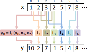
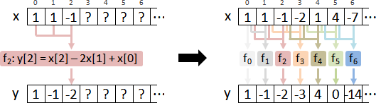
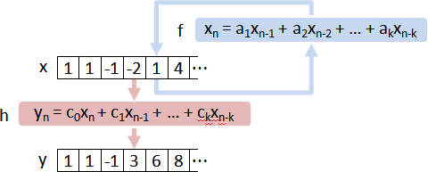
使用impulse response。
輸入是脈衝函數，輸出稱作脈衝響應。
LTI系統當中，脈衝響應恰是卷積核。
最後，卷積核進一步改寫成矩陣。

system realization原意是指找到系統模型、系統參數，以便建立系統。
由於訊號學家沒有考慮清楚，胡亂造詞、胡亂歸類。
system realization最終演變為完全不相干的意義：系統參數改寫成矩陣。

LTI system

state-space representation

線性函數（狹義版本）、線性遞迴函數，可以改寫成矩陣。

線性非時變系統的系統參數也可以改寫成矩陣，有兩種方式：
一、MIMO系統、線性非時變系統、一階。
　　改寫成矩陣，外觀仍是MIMO系統、一階。
　　將一個時刻的每種訊號併成向量。此向量是狀態。
　　經典應用是數值模擬的數值方案。
二、SISO系統、線性非時變系統、n階。
　　改寫成矩陣，外觀變成MIMO系統、一階。
　　將連續n個訊號數值併成向量。此向量是滑動視窗。
　　經典應用是遞迴數列的快速冪演算法。
此處使用二。
然而訊號學家卻將二稱作狀態空間表示法。成為歷史共業。

companion matrix realization

高階差分方程式，化作一階差分方程組。
高階微分方程式，化作一階微分方程組。

統計學與訊號學的差分方程式，
包括了輸入訊號和輸出訊號。

數學的差分方程式，
只有一個未知函數：對應到AR model。
恰有兩個未知函數：對應到ARMA model。

AR model:
x⃗[n+1] = A x⃗[n]

ARMA model:
x⃗[n+1] = A x⃗[n] + b

我思忖著通通改成b和y。【尚待確認】

AR(3) model:

   x[n+3] + a₂ x[n+2] + a₁ x[n+1] + a₀ x[n] = 0

=> x[n+3] = - a₂ x[n+2] - a₁ x[n+1] - a₀ x[n]

=> x+⃡3 = - a₂(x+⃡2) - a₁(x+⃡1) - a₀x      number -> sequence

   ⎧ (x  )+⃡1 = x+⃡1                      3rd-order equation
=> ⎨ (x+⃡1)+⃡1 = x+⃡2                      -> 1st-order system 
   ⎩ (x+⃡2)+⃡1 = - a₂(x+⃡2) - a₁(x+⃡1) - a₀x

   ⎧ x₀+⃡1 = x₁
=> ⎨ x₁+⃡1 = x₂                          rename variables
   ⎩ x₂+⃡1 = -a₂x₂ - a₁x₁ - a₀x₀

   ⎡ x₀+⃡1 ⎤   ⎡  0   1   0  ⎤ ⎡ x₀ ⎤    matrix representation
=> ⎢ x₁+⃡1 ⎥ = ⎢  0   0   1  ⎥ ⎢ x₁ ⎥    (companion matrix)
   ⎣ x₂+⃡1 ⎦   ⎣ -a₀ -a₁ -a₂ ⎦ ⎣ x₂ ⎦

=>   x⃗+⃡1    =        A          x⃗       rename variables

=>  x⃗[n+1]  =        A         x⃗[n]     sequence -> number

AR(5) model:

⎡ x₀+⃡1 ⎤   ⎡  0   1   0   0   0  ⎤ ⎡ x₀ ⎤
⎢ x₁+⃡1 ⎥   ⎢  0   0   1   0   0  ⎥ ⎢ x₁ ⎥
⎢ x₂+⃡1 ⎥ = ⎢  0   0   0   1   0  ⎥ ⎢ x₂ ⎥
⎢ x₃+⃡1 ⎥   ⎢  0   0   0   0   1  ⎥ ⎢ x₃ ⎥
⎣ x₄+⃡1 ⎦   ⎣ -a₀ -a₁ -a₂ -a₃ -a₄ ⎦ ⎣ x₄ ⎦

3rd-order linear differential equation:

   d³            d²            d
   ——— x(t) + a₂ ——— x(t) + a₁ —— x(t) + a₀ x(t) = 0
   dt³           dt²           dt

=> x‴(t) + a₂ x″(x) + a₁ x′(x) + a₀ x(t) = 0

=> x‴(t) = - a₂ x″(t) - a₁ x′(t) - a₀ x(t)

   ⎧ (x )′ = x′                       3rd-order equation
=> ⎨ (x′)′ = x″                       -> 1st-order system
   ⎩ (x″)′ = -a₂x″ - a₁x′ - a₀x

   ⎧ x₀′ = x₁
=> ⎨ x₁′ = x₂                         rename variables
   ⎩ x₂′ = -a₂x₂ - a₁x₁ - a₀x₀

   ⎡ x₀′ ⎤   ⎡  0   1   0  ⎤ ⎡ x₀ ⎤   matrix representation
=> ⎢ x₁′ ⎥ = ⎢  0   0   1  ⎥ ⎢ x₁ ⎥   (companion matrix)
   ⎣ x₂′ ⎦   ⎣ -a₀ -a₁ -a₂ ⎦ ⎣ x₂ ⎦

=>   x⃗′    =        A          x⃗      rename variables

similarity transformation

拿任意一種可逆矩陣T做相似變換。
   decomposition             A = TA'T⁻¹
=> similarity transformation A' = T⁻¹AT

對角化也是一種相似變換。變換矩陣是特徵向量。

minimal realization

數學稱作正則化canonicalization。
物理學稱作解耦合decoupling。
訊號學稱作最小實現minimal realization。
三者概念相同，只是著重的事情稍微有點差別。

總之一句話：矩陣對角化。
   eigendecomposition A = EΛE⁻¹
=> diagonalization    Λ = E⁻¹AE
變換矩陣A實施相似變換成為對角矩陣A' = Λ = E⁻¹AE。
對角線就是特徵值。將零集中在右下角。
最後去掉特徵值是零的多餘維度。

當A是同伴矩陣companion matrix。
特徵向量E恰是多項式內插矩陣Vandermonde matrix的轉置。

companion matrix:
    ⎡  0   1   0  ⋯  0    ⎤
    ⎢  0   0   1  ⋯  0    ⎥
A = ⎢  0   0   0  ⋯  0    ⎥
    ⎢  0   0   0  ⋯  1    ⎥
    ⎣ -a₀ -a₁ -a₂ ⋯ -aₙ₋₁ ⎦

eigenproblem:
Ax = λx

eigendecomposition:
A = EΛE⁻¹

eigenvalues:
λ₁, λ₂, ⋯, λₙ

eigenvectors:
    ⎡ λ₁⁰   λ₂⁰   ⋯ λₙ⁰   ⎤
    ⎢ λ₁¹   λ₂¹   ⋯ λₙ¹   ⎥    transpose of 
E = ⎢ λ₁²   λ₂²   ⋯ λₙ²   ⎥    Vandermonde matrix
    ⎢ :     :       :     ⎥
    ⎣ λ₁ⁿ⁻¹ λ₂ⁿ⁻¹ ⋯ λₙⁿ⁻¹ ⎦

表格

                         AR model
╭────────────────────────────┬────────────────────────────╮
│ polynomial representation  │ matrix representation      │
╞════════════════════════════╧════════════════════════════╡
│ time domain                                             │
│ impulse response representation                         │
╞════════════════════════════╤════════════════════════════╡
│ sequence                   │ companion matrix           │
│ b = (b[0], b[1], b[2], ⋯)  │     ⎡    0     1     0  ⋯ ⎤│
│                            │     ⎢    0     0     1  ⋯ ⎥│
│                            │ A = ⎢    0     0     0  ⋯ ⎥│
│                            │     ⎢    :     :     :    ⎥│
│                            │     ⎣ -b[0] -b[1] -b[2] ⋯ ⎦│
├────────────────────────────┤────────────────────────────┤
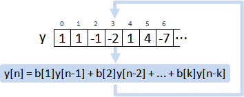
│ linear recurrence          │ linear recurrence          │
│ y[n] = b[1] y[n-1]         │ y⃗[n] = A y⃗[n-1]            │
│      + b[2] y[n-2]         │                            |
│      + ...                 │                            │
├────────────────────────────┤────────────────────────────┤
│ expansion                  │ expansion                  │
│ y[n] = .......             │ y⃗[n] = Aⁿ y⃗[0]             │
├────────────────────────────┤────────────────────────────┤
│ convolution                │ Toeplitz matrix            │
│ (y+⃡1) = b * y              │ (y⃗+⃡1) = 𝐺 y⃗                │
│                            │                            │
│                            │     ⎡ b[0]   0    0  ⋯  ⎤  │
│                            │     ⎢ b[1] b[0]   0  ⋯  ⎥  │
│                            │ 𝐺 = ⎢ b[2] b[1] b[0] ⋯  ⎥  │
│                            │     ⎢ b[3] b[2] b[1] ⋯  ⎥  │
│                            │     ⎣   :    :    :     ⎦  │ 
├────────────────────────────┤────────────────────────────┤
│ solution                   │ solution                   │
│ f[n] = C₀ 𝑝₀ⁿ              │ f[n] = C₀ Aⁿ               │
│      + C₁ 𝑝₁ⁿ              │                            │
│      + ...                 │                            │
╞════════════════════════════╧════════════════════════════╡
│ frequency domain                                        │
│ transfer function representation                        │
╞════════════════════════════╤════════════════════════════╡
│ generating function        │ matrix pencil              │
│ F(z) = f[0] z              │ zI-A                       │
│      + f[1] z⁻¹            │                            │
│      + ...                 │                            │
├────────────────────────────┤────────────────────────────┤
│ characteristic equation    │ characteristic equation    │
│ F(λ) = 0                   │ det(λI-A) = 0              │
|                            |                            |
│ λⁿ = f[1] λⁿ⁻¹             │                            │
│    + f[2] λⁿ⁻¹             │                            │
│    + ...                   │                            │
├────────────────────────────┤────────────────────────────┤
│ roots (poles)              │ eigenvalues (poles)        │
│ λ₁, λ₂, ...                │ λ₁, λ₂, ...                │
╰────────────────────────────┴────────────────────────────╯

LTI state-space system

專著《Filtering and System Identification: A Least Squares Approach》。

state-space representation

⎰ x⃗[n+1] = A x⃗[n] + B u⃗[n]
⎱ y⃗[n]   = C x⃗[n] + D u⃗[n]

LTI state-space system的四串系統參數也可以改寫成四個矩陣ABCD。【尚待確認】
但是教科書一律直接改寫成矩陣。完全見不到系統參數。

companion matrix realization

ARMA model可以進一步變成state-space model，湊出矩陣ABCD。

https://people.duke.edu/~hpgavin/SystemID/CourseNotes/LTI.pdf

similarity transformation

A' = T⁻¹AT
B' = T⁻¹B
C' = CT
D' = D
x' = T⁻¹x
u' = u
y' = y

eigensystem realization

eigensystem realization (Ho–Kálmán realization)

1. get (g[1], ⋯, g[n])
   by impulse response

2. get 𝑂,𝐶
   by compact SVD of Hankel((g[1], ⋯, g[n]))

3. get A,B,C,D
   A: extract from Hankel((g[2], ⋯, g[k+1]))
   B: first column of 𝐶
   C: first row of 𝑂
   D: orignal D (by similarity transformation)

https://math.stackexchange.com/questions/3275985/
https://par.nsf.gov/servlets/purl/10312038

reachability matrix / observability matrix

可到達性矩陣：x[n+1]遞迴函數，改寫成矩陣。
可觀察性矩陣：y[n]遞迴函數，改寫成矩陣。

藉由同伴矩陣，
訊號從數值x[n] y[n] z[n]推廣為向量u⃗[n] x⃗[n] y⃗[n]。
k是向量維度。k也是差分方程式的階數。
rank(A) = k，那麼A的直條的線性組合，得以形成每一種k維向量。
注意到，數列索引值n／數列長度n、向量維度k，兩者意義不同。

簡單起見，這個小節的u x y不添加向量符號、也不使用粗體字。

expansion of x (polynomial representation):

⎧ x[1] = A x[0] + B u[0]
⎨ x[2] = A² x[0] + AB u[0] + B u[1]
⎪   :
⎩ x[k] = Aᵏ x[0] + Aᵏ⁻¹B u[0] + ⋯ + AB u[k-2] + B u[k-1]

formula of x (matrix representation):

                                      ⎡ u[0]   ⎤
x[k] = Aᵏ x[0] + [ Aᵏ⁻¹B ⋯ A²B AB B ] ⎢   :    ⎥
                                      ⎣ u[k-1] ⎦
                           Ɔ

reachability matrix (controllability matrix):

𝐶 = [ A⁰B ⋯ Aᵏ⁻¹B ]

reachability:

    any y can be generated by x[0] and u
<=> any x[k] can be generated by x[0] and u[0⋯k-1]
<=> rank(𝐶) = k

expansion of y (polynomial representation):

⎧ y[0] = C x[0] + D u[0]
⎨ y[1] = CA x[0] + CB u[0] + D u[1]
⎪   :
⎩ y[k-1] = CAᵏ⁻¹ x[0] + CAᵏ⁻²B u[0] + ... + CAB u[k-1] + D u[k-1]

expansion of y (matrix representation):

⎡ y[0]   ⎤   ⎡ C     ⎤        ⎡ D    0   ⋯ ⎤ ⎡ u[0]   ⎤
⎢   :    ⎥ = ⎢ CA    ⎥ x[0] + ⎢ CB   D   ⋯ ⎥ ⎢   :    ⎥
⎢   :    ⎥   ⎢  :    ⎥        ⎢ CAB  CB  ⋯ ⎥ ⎢   :    ⎥
⎣ y[k-1] ⎦   ⎣ CAᵏ⁻¹ ⎦        ⎣ :    :     ⎦ ⎣ u[k-1] ⎦
                 𝑂                   𝐺

observability matrix:

    ⎡ CA⁰   ⎤
𝑂 = ⎢  :    ⎥
    ⎣ CAᵏ⁻¹ ⎦

observability:

    unique x can be reconstructed by y and u
<=> unique x[0] can be reconstructed by y[0⋯k-1] and u[0⋯k-1]
<=> rank(𝑂) = k

Krylov subspace：湊足k種連續次方，得以構成k維空間。
一、可到達性矩陣、可觀察性矩陣至少需要列出0次方到k-1次方。
二、訊號長度至少是k個數字，得以檢查可到達性、可觀察性。

Markov parameters

卷積核（脈衝響應）改寫成矩陣。然後省略g[0]。

Markov parameters:

(CA⁰B, CA¹B, ...)

theorem:

Hankel((g[1], ⋯, g[k])) = Hankel((CA⁰B, ⋯, CAᵏ⁻¹B)) = 𝑂𝐶

⎡ g[1] g[2]   ⋯ g[k]    ⎤   ⎡ CA⁰B   CA¹B ⋯ CAᵏ⁻¹B  ⎤
⎢ g[2] g[3]   ⋯ g[k+1]  ⎥   ⎢ CA¹B   CA²B ⋯ CAᵏB    ⎥
⎢   :    :        :     ⎥ = ⎢  :      :      :      ⎥ = 𝑂𝐶
⎢   :    :        :     ⎥   ⎢  :      :      :      ⎥
⎣ g[k] g[k+1] ⋯ g[2k-1] ⎦   ⎣ CAᵏ⁻¹B CAᵏB ⋯ CA²ᵏ⁻²B ⎦

Toeplitz matrix = constant diagonal matrix
Hankel matrix = constant skew-diagonal matrix

可到達性矩陣故意被左右顛倒，就是為了產生常反對角矩陣。
如果我沒搞錯，這與卷積互相呼應。
卷積的其中一個數列也是需要左右顛倒。

Hankel singular values

Hankel((g[1], ⋯, g[n]))
做共軛分解conjugate decomposition，得到𝑂與𝐶。
從中間剖開一人分一半。

共軛分解採用compact SVD，順便降維，以便形成minimal realization。
去掉奇異值是零的多餘維度。
方便起見，新維度還是標記成k，新矩陣則追加下標k。
A = UΣVᵀ = U√Σ√ΣVᵀ  compact singular value decomposition
Aₖ = Uₖ√Σₖ√ΣₖVₖᵀ    minimal realization (rank k)
𝑂 = Uₖ√Σₖ
𝐶 = √ΣₖVₖᵀ

A = BᵀB。
對稱半正定矩陣A，分解成矩陣內積。
沒有正式學術名稱。
少數文獻稱作共軛分解conjugate decomposition。
概念宛如將一個平方值，分解成共軛複數相乘。
分解方式有無限多種。其中有兩種知名方式：
一、Cholesky decomposition，分解成上三角矩陣。
    A = LLᵀ and B = Lᵀ
二、eigendecomposition。特徵分解。
    A = EΛE⁻¹ = EΛEᵀ = E√Λ√ΛEᵀ and B = √ΛEᵀ
對稱半正定矩陣的情況下，特徵分解EVD等同奇異值分解SVD！
不是對稱半正定矩陣的情況下，只好改用SVD。
Hankel((g[1], ⋯, g[k]))是對稱矩陣，但是通常不是半正定矩陣。

system matrices

算A：移位一個時刻，湊出A。然後𝑂和𝐶移項即得。
⎡ g[2]   g[3]   ⋯ g[k+1] ⎤   ⎡ CA¹B CA²B   ⋯ CAᵏB    ⎤
⎢ g[3]   g[4]   ⋯ g[k+2] ⎥   ⎢ CA²B CA²B   ⋯ CAᵏ⁺¹B  ⎥
⎢   :      :        :    ⎥ = ⎢  :      :      :      ⎥ = 𝑂A𝐶
⎢   :      :        :    ⎥   ⎢  :      :      :      ⎥
⎣ g[k+1] g[k+2] ⋯ g[2k]  ⎦   ⎣ CAᵏB CAᵏ⁺¹B ⋯ CA²ᵏ⁻¹B ⎦

let Hₖ = Hankel((g[1], ⋯, g[k]))
Aₖ = 𝑂ₖ⁺(Hₖ+⃡1)𝐶ₖ⁺

算B：𝐶ₖ第零個直條就是Bₖ。
算C：𝑂ₖ第零個橫條就是Cₖ。
算D：原本的D降維。【尚待確認】

balanced realization

balanced realization

四個矩陣ABCD的方程組，對角化比較複雜。
四個矩陣不能一起對角化。
只能以𝐶為主、或者以𝑂為主。

有人發現取平方（矩陣內積和外積）再開根號，𝐶和𝑂就可以一起對角化。
宛如SVD的背後原理。SVD即是EVD取平方（矩陣內積和外積）再開根號。

1. get P,Q by Lyapunov equation
   AP + PAᵀ + BBᵀ = 0
   AᵀQ + QA + CᵀC = 0
2. get 𝑂 by Cholesky decomposion
   Q = 𝑂ᵀ𝑂
3. get U,Σ by eigendecomposition
   𝑂P𝑂ᵀ = 𝑂𝐶𝐶ᵀ𝑂ᵀ= HHᵀ = UΣ²Uᵀ
4. get T by conjugate decomposition 
   T   = 𝑂⁻¹U√Σ
   T⁻¹ = √ΣUᵀ𝑂

其實步驟1和2是多餘的。
H = Hankel((g[1], ⋯, g[k]))
使用矩陣內積HᵀH、矩陣外積HHᵀ，即可完成平衡實現。
步驟1和2主要是為了介紹Lyapunov equation。

https://ocw.mit.edu/courses/6-241j-dynamic-systems-and-control-spring-2011/7f6754029d6945bd3bdc745080890bf8_MIT6_241JS11_chap26.pdf

image

線性代數當中，
image：一個矩陣，嘗試各種輸入向量，所能得到的各種輸出向量。輸出向量的集合。

theorem:
image(AAᵀ) = image(A)

直觀解讀：
一、Aᵀx是輸入向量x實施變換，獲得一部分的輸入向量。比原本少。
　　再經過A變換，獲得一部分的輸出向量。比原本少。
　　因此image(AAᵀ) ⊆ image(A)。
二、Aᵀ是垂直投影。Aᵀ消滅的維度，A消滅的維度，基本相等。
　　換句話說，rank(Aᵀ) = rank(A)。
　　即便額外套用Aᵀ，剩下的維度還是一樣多。
　　因此image(AAᵀ) = image(A)。

嚴謹證明，分成三個階段：
(1) AᵀAx = 0 <=> Ax = 0
(2) kernel(AᵀA) = kernel(A)
(3) image(AᵀA) = image(Aᵀ)

(1)(⟹) 等號兩邊同乘xᵀ
   AᵀAx = 0
=> xᵀAᵀAx = 0
=> ‖Ax‖² = 0
=> Ax = 0

(1)(⟸) 等號兩邊同乘Aᵀ。
   Ax = 0
=> AᵀAx = 0

(2) 因為兩個方程式等價，所以兩個解集合也等價。

(3) 線性代數基本定理：kernel(A) = image(Aᵀ)⟂
   kernel(AᵀA) = kernel(A)
=> image((AᵀA)ᵀ)⟂ = image(Aᵀ)⟂
=> image(AᵀA)⟂ = image(Aᵀ)⟂
=> image(AᵀA) = image(Aᵀ)

https://math.stackexchange.com/questions/2411508

reachability

圖論當中，
reachable：從一個起點可以到達一個終點。
connected：從各種起點可以到達各種終點。

訊號學當中，
reachable set：從各種起點所能到達的各種終點。終點的集合。

使用矩陣來描述相鄰關係，
訊號學的reachable set＝線性代數的image。

先備知識請見本站文件「adjacency matrix」。
圖論當中，A是圖。Aᵀ是反向圖（顛倒所有邊）。
套用Aᵀ：順走1步。
套用A：逆走1步。
套用AAᵀ：先順走1步、再逆走1步（矩陣乘法由右往左讀）。

考慮所有可能的起點，以及所有可以到達的終點。
套用A、套用AAᵀ，所有可以到達的終點一樣多。

套用R = (A⁰+A¹+⋯+Aᵏ)：
逆走0步到k步，所到之處通通聯集。
套用RRᵀ = (A⁰+A¹+⋯+Aᵏ)(A⁰+A¹+⋯+Aᵏ)ᵀ：
先順走再逆走（矩陣乘法由右往左讀）。
展開式子，變成兩兩相乘，得到各種情況。例如順1逆2。
套用P = A⁰(A⁰)ᵀ+A¹(A¹)ᵀ+⋯+Aᵏ(Aᵏ)ᵀ：
順0逆0、順1逆1、……、順k逆k，所到之處通通聯集。

考慮所有可能的起點，以及所有可以到達的終點。
套用R、套用P，所有可以到達的終點一樣多。

reachability Gramian

Gram matrix            MᵀM

k-step                 Aᵏ⁻¹B
outer product          (Aᵏ⁻¹B)(Aᵏ⁻¹B)ᵀ = Aᵏ⁻¹BBᵀ(Aᵏ⁻¹)ᵀ
image                  image(Aᵏ⁻¹B) = image((Aᵏ⁻¹B)(Aᵏ⁻¹B)ᵀ)

k-reachability matrix         𝐶ₖ = [ A⁰B ⋯ Aᵏ⁻¹B ]
k-reachability Gramian matrix [ A⁰BBᵀ(A⁰)ᵀ ⋯ Aᵏ⁻¹BBᵀ(Aᵏ⁻¹)ᵀ ]

k-reachability         R[k] = sum Aᵏ⁻¹B
                             k=0⋯∞
k-reachability Gramian P[k] = sum Aᵏ⁻¹BBᵀ(Aᵏ⁻¹)ᵀ = sum 𝐶ₖ 𝐶ₖᵀ
                             k=0⋯∞                k=0⋯∞
k-reachable set        image(R[k]) = image(P[k])

https://control.asu.edu/Classes/MAE507/507Lecture06.pdf
https://control.asu.edu/Classes/MAE507/507Lecture17.pdf

Lyapunov equation

k-reachability Gramian P[k+1] = A P[k] Aᵀ + BBᵀ
Lyapunov stability     image(P[k+1]) = image(P[k]) when k→∞
Lyapunov equation      M = AMAᵀ + BBᵀ
                       where M = P[k] and k→∞
Lyapunov theorem       Lyapunov stability <=> Lyapunov equation

Hankel singular value

reachability Gramian   P = 𝐶𝐶ᵀ  =>  AP + PAᵀ + BBᵀ = 0
observability Gramian  Q = 𝑂ᵀ𝑂  =>  AᵀQ + QA + CᵀC = 0
Hankel singular value  Σ = sqrt(eigenvalue(PQ))
balanced realization   P' = Q' = Σ

similarity transformation

P' = T⁻¹P(Tᵀ)⁻¹
Q' = TᵀQT

延伸閱讀：dual system

rank / nullity

矩陣尺寸是n，而實際維度不足n。
套用此矩陣、實施變換，有些維度完全消失。
例如投影矩陣，有些維度完整保留，有些維度完全消失。
消失的維度，特徵值是零，特徵向量未定義。
（數學家規定必須湊滿n個特徵值。但是不必湊滿n個特徵向量。）

stability / instability

繼續深入。
實際維度是k，其中包含了縮小、不變、放大。
矩陣尺寸是n，其中包含了消失、縮小、不變、放大。
特徵值，其中包含了等於0，絕對值小於1、絕對值等於1、絕對值大於1。
不斷套用此矩陣、不斷實施變換，
有些維度完全消失、趨近消失、保持不變、變成正負無限大。

消失、縮小、不變，最終形成穩態。
放大，最終不會形成穩態。

reachability / controllability / stabilizability

可到達性：已知初始狀態x[0]，
　　　　　總是存在控制訊號u，可以得到每一種當前狀態x[n]。
　　　　（可以得到每一種狀態數列x。畢竟已知系統公式。）
可控制性：已知初始狀態x[0]、當前狀態x[n]。
　　　　　總是存在控制訊號u，可以得到當前狀態x[n]。
　　　　（可以得到狀態數列x、輸出數列y。畢竟已知系統公式。）
可穩定性：已知初始狀態x[0]，
　　　　　總是存在控制訊號u，使得每種輸出訊號y到達穩態。
　　　　（即便不滿足可控制性。例如ABCD矩陣全是零。）

一般來說，可到達性=>可控制性。
有反矩陣，可到達性<=>可控制性。

現實當中，有可能不可到達、但是可控制。
舉例來說，一部分特徵值是零，
輸入訊號剛好落在這些特徵向量構成的子空間，糊里糊塗得到零。
你也只能得到零，無法得到其他東西。

observability / constructability / detectability

可觀察性：已知輸出訊號y、控制訊號u，
　　　　　可以得到唯一一種初始狀態x[0]。
　　　　（可以得到唯一一種狀態數列x。畢竟已知系統公式。）
可建設性：已知輸出訊號y、控制訊號u、當前狀態x[n]。
　　　　　可以成立。
可偵測性：已知輸出訊號y、控制訊號u，
　　　　　可以讓輸出訊號y到達穩態。
　　　　（即便不滿足可觀察性。例如不知道狀態但知道會穩定。）

一般來說，可觀察性=>可建設性。
有反矩陣，可觀察性<=>可建設性。

現實當中，有可能不可觀察、但是可建設。
homogeneous solution多解的部分剛好可逆。

output controllablility

output controllable if and only if the output controllability
Gramian is positive definite.

https://arxiv.org/pdf/2306.08523

dual system

四個矩陣ABCD通通轉置，仍然是LTI state-space system。
四個矩陣ABCD通通轉置，reachability與observability恰好對調。
原理是線性代數基本定理：kernel(A) = image(Aᵀ)⟂
就這樣。

controllable canonical form / observable canonical form

以矩陣A為主角，
實施companion matrix realization，
得到controllable canonical form。

四個矩陣ABCD通通轉置，得到另外一種canonical form。
即是dual system。

http://www.dii.unimo.it/~zanasi/didattica/Teoria_dei_Sistemi/Luc_TDS_ING_2016_Reachability_and_Controllability.pdf
http://www.dii.unimo.it/~zanasi/didattica/Teoria_dei_Sistemi/Luc_TDS_ING_2016_Observability_and_Constructability.pdf

表格

專著《Linear Optimal Control: H₂ and H_∞ Methods》。

                  LTI state-space system
╭────────────────────────────┬────────────────────────────╮
│ polynomial representation  │ matrix representation      │
╞════════════════════════════╧════════════════════════════╡
│ time domain                                             │
│ impulse response representation                         │
╞════════════════════════════╤════════════════════════════╡
│ sequence                   │ companion matrix           │
│ a,b,c,d                    │ A,B,C,D                    │
│ a = (a[0], a[1], ...)      │                            │
│ b = (b[0], b[1], ...)      │                            │
│ c = (c[0], c[1], ...)      │                            │
│ d = (d[0], d[1], ...)      │                            │
├────────────────────────────┤────────────────────────────┤
│ linear recurrence          │ linear recurrence          │
│ ⎧ x[n+1] = a[0] x[n] + ⋯   │ ⎰ x⃗[n+1] = A x⃗[n] + B u⃗[n] │
│ ⎨        + b[0] u[n] + ⋯   │ ⎱ y⃗[n]   = C x⃗[n] + D u⃗[n] │
│ ⎪ y[n]   = c[0] x[n] + ⋯   │                            │
│ ⎩        + d[0] u[n] + ⋯   │                            │
├────────────────────────────┤────────────────────────────┤
│ expansion                  │ expansion                  │
│ x[n+1] = ......            | x[n+1] = Aⁿ⁺¹ x[0] + Ɔ u⃗[n]|
│ y[n]   = ......            │ y⃗[n]   = 𝑂 x[0] + 𝐺 u⃗[n]   │
├────────────────────────────┤────────────────────────────┤
│ convolution                │ Hankel matrix              │
│ ⎰ x+⃡1 = a ∗ x + b ∗ u      │ 𝑂𝐶                         │
│ ⎱ y   = c ∗ x + d ∗ u      │                            │
├────────────────────────────┤────────────────────────────┤
│ impulse response           │ Markov parameters          │
│ g[n] = ......              │ g[n] = CAⁿ⁻¹B + D δ[n]     │
│                            │      = ⎰ D      , if n = 0 │
│                            │        ⎱ CAⁿ⁻¹B , if n > 0 │
├────────────────────────────┤────────────────────────────┤
│ solution                   │ solution                   │
│ y[n] = ......              │ y[n] = C Aⁿ x[0]           │
│                            │      +  sum  CAⁿ⁻¹⁻ⁱB u[i] │
│                            │       i=0⋯n-1              │
│                            │      + D u[0]              │
╞════════════════════════════╧════════════════════════════╡
│ frequency domain                                        │
│ transfer function representation                        │
╞════════════════════════════╤════════════════════════════╡
│ generating function        │ resolvent                  │
│ A(z) = a[0]z + a[1]z⁻¹ + ⋯ │ G(z) = C(zI-A)⁻¹B + D      │
│ B(z) = b[0]z + b[1]z⁻¹ + ⋯ │          adj(zI-A)         │
│ C(z) = c[0]z + c[1]z⁻¹ + ⋯ │      = C ————————— B + D   │
│ D(z) = d[0]z + d[1]z⁻¹ + ⋯ │          det(zI-A)         │
├────────────────────────────┤────────────────────────────┤
│ BIBO stability             │ BIBO stability             │
│ A(λ) = 0                   │ det(λI-A) = 0              │
├────────────────────────────┤────────────────────────────┤
│ roots (poles)              │ eigenvalues (poles)        │
│ λ₁, λ₂, ...                │ λ₁, λ₂, ...                │
╰────────────────────────────┴────────────────────────────╯

system functionality

不知道該下什麼標題才好。

「系統功能」。系統是函數、甚至是函數網路。工程師設計函數網路，達成特定任務，例如生成／濾波／觀測／控制。

生成器：沒有輸入訊號，輸出一道訊號。
　　　　需要設定參數。
濾波器：系統輸出之後，追加一個系統，用來調整輸出訊號。
　　　　需要設定參數。
觀測器：系統輸出之後，追加一個系統，用來觀測系統內部狀態。
　　　　輸入訊號需要前饋。
控制器：系統輸入之前，追加一個系統，用來調整輸入訊號暨輸出訊號。
　　　　輸出訊號需要回饋。

verb     | action noun | agent noun
---------|-------------|-----------
generate | generation  | generator
filter   | filter      | filter
observe  | observation | observer
control  | control     | controller

       ┌───────────┐
       │ generator │────→ x
       └───────────┘

       ┌──────────┐  y  ┌──────────┐
x ────→│  system  │────→│  filter  │────→ y'
       └──────────┘     └──────────┘

       ┌──────────┐
u ──┬─→│  system  │──┬──────────────────→ y
    │  └──────────┘  └─→┌──────────┐
    ╰──────────────────→│ observer │────→ x̂
                        └──────────┘

       ┌──────────┐  u  ┌──────────┐
r ────→│controller│────→│  system  │──┬─→ y
    ╭─→└──────────┘     └──────────┘  │
    ╰─────────────────────────────────╯

generator

「生成器」。函數，輸入參數，輸出訊號。

pulse generator / oscillator

脈衝生成器：產生三角形函數或者鐘形函數，寬度極窄，自訂寬度。
振盪器：產生週期函數。例如方波、三角波、鋸齒波、弦波。
實作方式採用程式語言，事情非常簡單。將數學函數直接寫成程式碼。
實作方式採用電子電路、生化反應，事情非常複雜。此處省略。

filter

low-pass filter / high-pass filter

濾波器只保留低頻波、只保留高頻波。

band-pass filter / band-stop filter

濾波器只保留中頻波、只刪除中頻波。

Shelving filter / Butterworth filter

濾波器保留低頻波或高頻波；其餘的波，頻率相差越遠、保留越少。比較平滑柔順啦。
濾波器保留中頻波；其餘的波，頻率相差越遠、保留越少。比較平滑柔順啦。
Shelving filter其實有時域公式喔！
http://www.cs.cf.ac.uk/Dave/CM0268/PDF/10_CM0268_Audio_FX.pdf

peak filter / notch filter

濾波器頻譜呈現一個尖峰、頻譜呈現一個尖谷。

difference filter / feedforward comb filter / feedback comb filter

延遲1刻  yn = xn + a xn-1
延遲d刻  yn = xn + a xn-d   （頻譜的振幅呈現連綿圓峰）
改成回饋 yn = xn + a yn-d   （頻譜的振幅呈現梳子）（連綿圓丘上下顛倒）

2nd-order其實就是延遲時刻有小數點，需要做線性內插。
https://thewolfsound.com/allpass-filter/

all-pass filter

濾波器頻譜，振幅不變（常數1）、相位改變。
例如feedforward comb filter與feedback comb filter串聯。
https://ccrma.stanford.edu/~jos/pasp/Allpass_Two_Combs.html

moving average filter

k點平均  yn = (xn + xn-1 + ... + xn-k+1) / k
（頻譜的振幅呈現連綿縮小圓丘）

window function / spectral leakage

傅立葉轉換，只有整數倍頻率波。
如果訊號不是整數倍頻率波所組成，那就完蛋了。
非整數倍頻率波，將分散到各個整數倍頻率波，漏的到處都是。
訊號預先乘以窗函數，才做傅立葉轉換，稍微有點療效。
窗函數也可以想成是一種濾波器：連綿圓丘，消滅非整數倍頻率波。

sampling / aliasing

取樣，連續波變離散波。
根據取樣定理，
頻率超過取樣頻率兩倍的連續波（高頻連續波、取樣間隔太大），
將得到頻率稍小的離散波（波長稍長）。
固定取樣頻率時，若上述連續波頻率增大，則上述離散波頻率減小。
從頻譜來看，差不多是往左鏡射、往左翻書，中譯疊頻。
解法是連續波事先做lowpass filter。
去除高頻連續波，讓它沒有東西用來鏡射翻書。
但是濾波器無法做到完美矩形，只能陡降斜下。
稱作sharp cutoff lowpass filter。
曲線越陡價格越貴。

observer

estimation / prediction

估計：找到內部狀態。
預測：找到下個訊號。

找到迴歸函數之後，就可以預測訊號啦。
一旦獲得當前狀態，就可以估計下一個輸出訊號。
然後就可以計算誤差。

       ┌──────────┐
u ──┬─→│  system  │──┬───────────────────┬─→ y
    │  └──────────┘  └─→┌──────────┐  ŷ  │+
    ╰──────────────────→│ observer │────→╰─→ y - ŷ
                        └──────────┘    -

         ┌──────────┐ 
u ──┬───→│  system  │──┬──┬─→ y
    │    └──────────┘  │ +↓
    │ ╭────────────────╯  ├─→ y - ŷ
    │ ╰─→┌──────────┐    -↑
    └───→│ observer │─────┴─→ ŷ
         └──────────┘

Luenberger observer

x̂[n+1] = A x̂[n] + B u[n] + L (y[n] - ŷ[n])

找到一個幾乎一樣的LTI state-space system。

Luenberger observer不太流行。【尚待確認】
如果知道四個矩陣ABCD，即可遞推計算內部狀態x。不必繞圈子。
如果不知道四個矩陣ABCD，Luenberger observer不可靠。

追加u[n] = Fx̂[n]形成閉迴路。
整體也得滿足穩定性。
特徵值變成A+BF和A+LC。

     u        ┌──────────┐ 
 ┌───────┬───→│  system  │──┬─→ y
 │       │    └──────────┘  │
 │       │ ╭────────────────╯
u│       │ ╰─→┌──────────┐ x̂
 │       └───→│ observer │──┐
 │ ┌───┐      └──────────┘  │
 └─│ F │←───────────────────┘
   └───┘

https://www.columbia.edu/~ja3451/courses/E6602/9_observers.pdf
https://control.asu.edu/Classes/MAE507/507Lecture09.pdf

Kalman filter (linear quadratic estimator)

Kalman filter非常流行。
雖然是observer，但是原始作者取名filter。
畢竟當時observer這個詞彙尚未流行。

Kalman filter:
⎰ x[n+1] = A x[n] + B u[n]
⎱ y[n]   = C x[n]

使用測量儀器h，時時收集數據y，時時推敲現況x。推定現況是自迴歸系統f，合乎自然規律。自創測量儀器是系統h，合乎電路原理。根據結果，推敲原因，此行為稱作「線性二次估計linear quadratic estimation」。

I don't know the name 🚧

遞迴數列作為系統的輸入。
求解。求得原本遞迴數列。

resolution: ⎰ f(?) = ? +⃡ 1 , find x
            ⎱ h(?) = y

輸出誤差，通過反系統，得到輸入誤差，用以修正輸入。

為什麼要大費周章，將觀察值的誤差通過反系統，而不是直截了當，將觀察值通過反系統？我也不清楚。

h(x) = y
狀態 x₀ x₁ x₂ ...   未知（線性遞迴數列）
函數 h₀ h₁ h₂ ...   已知（數列每一項皆有一個函數）
觀察 y₀ y₁ y₂ ...   已知（數列每一項皆有一個輸出）

狀態是自迴歸模型    xₙ = f(xₙ₋₁, xₙ₋₂, ..., xₙ₋ₖ)
                    xₙ = a₁xₙ₋₁ + a₂xₙ₋₂ + ... + aₚxₙ₋ₖ

函數是平均值移動模型   yₙ = hₙ(xₙ, xₙ₋₁, xₙ₋₂, ..., xₙ₋ₚ)
                       yₙ = bₙ₀xₙ + bₙ₁xₙ₋₁ + ... + bₙₚxₙ₋ₚ

函數可以一樣        h₀ = h₁ = h₂ = ...

從 x₁ 開始一個一個算到 xᵢ，現在要算 xᵢ 是多少：

1. x̂ᵢ = f(xᵢ₋₁)              x 數列估計下一項。 (x₀ = 0)
                             此處以一階函數為例。

2. ŷᵢ = hᵢ(x̂ᵢ)               y 數列估計下一項。
　                           盜版 ŷᵢ 通常不等於正版 yᵢ。
                             這表示 x̂ᵢ 不夠準，需要修正。

3. kᵢ⁻¹                      求得誤差的反系統 kᵢ⁻¹。稱作Kalman gain。
                             kᵢ(x̂ᵢ - xᵢ) = (ŷᵢ - yᵢ)

 (1) pᵢ = (x̂ᵢ - xᵢ)²         為了計算反系統，需要 xᵢ 的誤差的平方。
        = cov(x̂ᵢ - xᵢ)       即是誤差的covariance。
     sᵢ = (ŷᵢ - yᵢ)²         不過由於我們還沒求出 xᵢ，所以不能這樣算。
        = cov(ŷᵢ - yᵢ)

 (2) p̂ᵢ = f²(pᵢ₋₁)           p 數列估計下一項。 (p₀ = 0)
        = f pᵢ₋₁ fᵀ          原理是 Var[k⋅X] = k² ⋅ Var[X]。

 (3) ŝᵢ = hᵢ²(p̂ᵢ)            s 數列估計下一項。
        = hᵢ p̂ᵢ hᵢᵀ          如果 f h 各有誤差項：常態分布 q r，平均數0。
                             那麼 p̂ᵢ ŝᵢ 各加上 var(q) var(r)。

 (4) kᵢ⁻¹ = p̂ᵢ hᵢᵀ ŝᵢ⁻¹      反系統是變異數的比值。這是什麼鬼啦？

4. xᵢ = x̂ᵢ - kᵢ⁻¹(ŷᵢ - yᵢ)   修正 x。
                             yᵢ 的誤差，通過反系統，還原成 xᵢ 的誤差。
                             x̂ᵢ 補上誤差，答案就對了。

5. pᵢ = p̂ᵢ - kᵢ⁻²(ŝᵢ)        修正 p。
      = p̂ᵢ - kᵢ⁻¹ ŝᵢ kᵢ⁻¹ᵀ

controller

controller應用十分廣泛，是世上最實用的演算法之一。

https://www.mathworks.com/solutions/control-systems/feedback-control-systems.html
https://ctms.engin.umich.edu/CTMS/index.php

(1) 系統名稱：LTI system
    主題名稱：linear control
    控制器名稱：PID controller
    數學工具：沒有。手動調參，稱作PID tuning。
(2) 系統名稱：LTI state-space system
    主題名稱：optimal control
    控制器名稱：linear quadratic regulator/tracker
    數學工具：quadratic optimization，求得公式解。

controller / plant

追加一個系統（控制器），用來控制原本系統（受控廠）。
控制器的輸出訊號，作為受控廠的輸入訊號。
控制器調整了輸入訊號，受控廠得到了特別的輸出訊號。

in practice:
                                    plant
                            ╭┄┄┄┄┄┄┄┄┄┄┄┄┄┄┄┄┄┄┄╮
reference ─┬─→ controller ─→┆actuator ─→ process┆──┬──→ output
           ↑                ╰┄┄┄┄┄┄┄┄┄┄┄┄┄┄┄┄┄┄┄╯  │
           └────────────── sensor ←────────────────┘

in theory:

reference ─┬─→ controller ──→ plant ──┬──→ output
           ↑                          ↓
           └──────────────←───────────┘

           　　　　  時域  頻域
reference  參考訊號  r(t)  R(s)
output     輸出訊號  y(t)  Y(s)
controller 控制器　  k(t)  K(s)
plant      受控廠　  g(t)  G(s)
actuator   致動器
process    程序
sensor     感測器　  h(t)  H(s)

regulation / tracking

輸出訊號趨近（固定不變的）固定數值
輸出訊號趨近（即時改變的）參考訊號

regulator:

     ┌──────────┐  u  ┌─────────┐
  ╭─→│controller│────→│  plant  │──┬─→ y
  │  └──────────┘     └─────────┘  │
  ╰────────────────────────────────╯

tracker:

     ┌──────────┐  u  ┌─────────┐
r ──→│controller│────→│  plant  │──┬─→ y
  ╭─→└──────────┘     └─────────┘  │
  ╰────────────────────────────────╯

LTI system

open-loop controller / closed-loop controller

open-loop controller:

 r ┌──────────┐ u ┌─────────┐ y
──→│controller│──→│  plant  │──→
   └──────────┘   └─────────┘

closed-loop controller:

 r   e=r-y ┌──────────┐ u ┌─────────┐  y
──→⊕──────→│controller│──→│  plant  │──┬─→
  -↑       └──────────┘   └─────────┘  │
   ╰───────────────────────────────────╯

開迴路控制：控制器的輸入是參考訊號。
閉迴路控制：控制器的輸入是誤差。
誤差是參考訊號減輸出訊號（跟統計學家的習慣相反）。
用膝蓋想也知道，誤差訊息量更多，於是效果更好。
其實兩者可以一併使用，尤其是非線性系統。
甚至沒有必要計算誤差，直接使用參考訊號與輸出訊號，尤其是多變數系統。
效果更好的正式說法是靈敏度較低：
(dT/T)/(dG/G)，控制系統變化與受控廠變化的比值。
教科書談靈敏度，喜歡以P controller的穩態誤差當作範例。只是在誤導大眾。

PID controller

e(t) = r(t) - y(t)     error

u(t) = kp e(t) + ki ∫ e(t) dt + kd d/dt e(t)   control
       ^^^^^^^   ^^^^^^^^^^^^   ^^^^^^^^^^^^   signal
    proportional   integral      derivative
     controller   controller     controller

y(t) = u(t) ∗ g(t)     output

proportion    比例。乘上某個百分比的結果。
integral      積分。積分運算的結果。
derivative    導數。微分運算的結果。

P controller：原值，再乘上權重kp。誤差當前數值。
I controller：積分，再乘上權重ki。誤差前綴和。過往累計。
D controller：微分，再乘上權重kd。誤差相鄰差。瞬間變化。

closed-loop PID controller (in theory):

───┬──→ kp + ki/s + kd*s ──→ G(s) ──┬──→
  -└───────────────←────────────────┘

rate feedback PID controller (in practice):

───┬──→ kp + ki/s ───────┬─→ G(s) ──┬──→
  -│                    -└── kd*s ←─┤
   └────────────────←───────────────┘

PID tuning

此處討論tracking。參考訊號是步進函數（目標數值是1，當前數值是0）。

此時大家觀察下述指標，評定優劣。
rising time     tr  到達1的時間（從0.1到0.9的時間，避免計入緩速時段）
settling time   ts  到達穩態的時間（保持在0.99到1.01之內）
peak time       tp  到達第一個局部極值的時間（最高峰）
peak overshoot  Mp  超過1的部分（最高峰減1，單位百分比）

此時PID controller調整參數，輸出訊號會有下述效果。
kp  調整斜率、改變頻率。增益（效果是放大縮小）。
ki  調整平均、改變穩態。高通濾波器（效果是鋸齒化）
kd  調整曲率、改變振幅。低通濾波器（效果是平滑化）。

Ziegler–Nichols tuning：古聖先賢發明了經驗公式。兩種調參方法。
1. quarter decay ratio
2. ultimate sensitivity method
https://my.ece.utah.edu/~ece3510/Notes_PID_Tuning_long.pdf

程式範例，受控廠是二次微分方程、0 zero 2 poles、-1 -2。

詳細圖解，位於影片後段。

stability analysis

專著《Linear Control System Analysis and Design: Conventional and Modern》。

pole–zero plot

極零圖：transfer function的poles與zeros。極Ｘ零Ｏ。
畫出poles和zeros的位置，以便判斷穩定性。
如果極Ｘ都在左半複平面（開區間、不含虛軸），則穩定。
如果右半複平面沒有極Ｘ（閉區間、包含虛軸），則穩定。

transfer function的poles，就是分母的zeros。
畫出分母的極零圖，亦可判斷穩定性。
如果右半複平面沒有零Ｏ，則穩定。

root locus plot

https://control.asu.edu/Classes/MAE318/318Lecture12.pdf

根軌跡圖：transfer function附帶一個參數（例如kp）。
窮舉參數值，畫出poles的變化軌跡，以便判斷穩定性。

1. open-loop controller:
r                u            y
───→ controller ──→ plant ────→
        K(s)         G(s)

transfer function:
K(s)G(s)

2. closed-loop controller:
r    e=r-y              u             y
───┬──────→ controller ──→ plant ──┬──→
  -↑           K(s)         G(s)   ↓
   └─────────────←─────────────────┘

transfer function:
  K(s)G(s)
————————————
1 + K(s)G(s)

3. 改寫成分式
K(s) = nᴋ(s) / dᴋ(s)
G(s) = nɢ(s) / dɢ(s)

transfer function:
  K(s)G(s)           nᴋ(s)nɢ(s)
———————————— = ———————————————————————
1 + K(s)G(s)   dᴋ(s)dɢ(s) + nᴋ(s)nɢ(s)

4. P controller:
K(s) = kp
nᴋ(s) = kp
dᴋ(s) = 1

transfer function:
  K(s)G(s)       kp G(s)         kp nɢ(s)             nɢ(s)     
———————————— = ——————————— = ———————————————— = ————————————————
1 + K(s)G(s)   1 + kp G(s)   dɢ(s) + kp nɢ(s)   dɢ(s)/kp + nɢ(s)

transfer function的poles，就是分母的根。
1 + kp G(s) = 0 或 dɢ(s) + kp nɢ(s) = 0 或 dɢ(s)/kp + nɢ(s) = 0
注意到，如果今天不是採用P controller，那麼需要重新推導。

現在要畫出transfer function的poles軌跡。kp = 0⋯∞。
當kp = [0,∞)，根軌跡是分母1 + kp G(s)的根。
當kp = 0，根軌跡起點恰是dɢ(s)的根，即是G(s)的poles。
當kp → ∞，根軌跡終點恰是nɢ(s)的根，即是G(s)的zeros。

採用P controller的情況下，K(s) = kp只是一個倍率。
此時G(s)的zeros/poles，
恰是open-loop transfer function K(s)G(s)的zeros/poles。
導致大家認為root locus的起點和終點就是開迴路的poles/zeros。
然而一般情況下根本無法牽扯到開迴路。成為歷史共業。

古聖先賢發明了手工製圖方法。好幾條規則。
https://www.mit.edu/people/klund/weblatex/node8.html

5. closed-loop controller with sensor:
r    e=r-y              u             y
───┬──────→ controller ──→ plant ──┬──→
  -↑           K(s)         G(s)   │
   │                               │
   └─────────── sensor ←───────────┘
                 H(s)

transfer function:
    K(s)G(s)
————————————————
1 + K(s)G(s)H(s)

教科書定義K(s)G(s)H(s) = k L(s)，但是內文根本沒有用到。來亂的。

Nyquist plot

https://lpsa.swarthmore.edu/Nyquist/NyquistStability.html
https://ocw.mit.edu/courses/18-04-complex-variables-with-applications-spring-2018/44f1db513a6a17d655abe0b6ff7748fc_MIT18_04S18_topic11.pdf

Nyquist圖：實施下述變換。
輸入：圍線（封閉路徑）（點集合），順時針圍住右半複平面。s = (-𝑖∞,+𝑖∞)
函數：逐點對應，s -> 1+K(s)G(s)。
輸出：新圍線。稱作Nyquist圖。
總結：右半複平面圍線，每一點s計算1+K(s)G(s)，逐點描繪新圍線。
性質：s = (-𝑖∞,0]與s = [0,+𝑖∞)的新圍線呈上下鏡面對稱。
取巧：加一就是圍線往右位移。大家習慣畫K(s)G(s)，再用-1取代原點。
取巧：當K(s) = kp，大家習慣畫G(s)，再用-1/kp取代-1。

Cauchy's integral theorem：
複變函數f(z)，圍線積分路徑圍住零個洞，圍線積分是0。

Cauchy's residue theorem：
複變函數f(z)，圍線積分路徑圍住多個洞，圍線積分是2π𝑖乘上留數和。

Cauchy's argument principle：
複變函數f′(z)/f(z)，圍線積分路徑圍住P個極、Z個零，圍線積分是2π𝑖(Z-P)。
援引winding number，上述圍線積分重新視作逆時針繞圈(Z-P)次。

Cauchy's argument principle：
複變函數f(z)，有多個極零。
一條圍線，逆時針繞圈一次，圍住P個poles、Z個zeros，
該條圍線實施f(z)變換之後，
一條圍線，逆時針繞圈(Z-P)次，圍住原點。

Nyquist stability criterion：
閉迴路系統極零圖，右半複平面不含閉迴路系統的pole，則穩定。
閉迴路系統K(s)G(s)/(1+K(s)G(s))的pole，就是分母1+K(s)G(s)的zero。
分母1+K(s)G(s)，有多個極零。
分母極零圖，右半複平面不含分母1+K(s)G(s)的zero，則穩定。
分母極零圖，右半複平面圍線，沒有圍住分母1+K(s)G(s)的zero，則穩定。
分母極零圖，令右半複平面有P個pole、Z個zero，令圍線是逆時針。
Nyquist圖，逆時針繞圈(-P)次，且圍住原點，則Z=0，則穩定。
（必須事先知道P是多少。因此此定理不實用。）

分母極零圖，右半複平面圍線，習慣畫順時針。
Nyquist圖，習慣畫K(s)G(s)而非1+K(s)G(s)，用-1取代原點。
Nyquist圖，逆時針繞圈P次，且圍住-1，則穩定。

採用P controller的情況下，K(s) = kp只是一個倍率。
Nyquist圖，習慣畫G(s)而非K(s)G(s)，用-1/kp取代-1。
Nyquist圖，逆時針繞圈P次，且圍住-1/kp，則穩定。

兩種製圖方式。
一、已知系統，以紙筆計算：
　　先畫波特圖（頻譜），再依此畫Nyquist圖。
　　s = (-𝑖∞,+𝑖∞)恰好對應傅立葉轉換的每種頻率的波。
二、未知系統，以儀器測量：
　　大家假設K(s)G(s)的pole比zero數量多、分母比分子次方高，
　　當s → ∞，則分母1+K(s)G(s) → 1。Nyquist圖可以畫得出來。
　　即便系統不穩定，Nyquist圖在下述情況還是畫得出來：
　　分母極零圖，右半複平面圍線，沒有途經分母1+K(s)G(s)的zero。
　　也就是說，閉迴路系統的pole不在虛軸上面。

Bode plot

https://lpsa.swarthmore.edu/Bode/BodeReviewRules.html

波特圖：系統的頻譜。分為振幅頻譜和相位頻譜。
振幅頻譜：採用log-log plot。橫軸頻率取log、縱軸振幅取log。
相位頻譜：採用semi-log plot。橫軸頻率取log、縱軸角度。

Bode stability criterion：
if open-loop K(s)G(s) is stable
and |K(s)G(s)| < 1 for all s: ∠K(s)G(s) ≡ 180° (mod 360°)
then closed-loop (K(s)G(s))/(1+K(s)G(s)) is stable.
先看相位頻譜，-180°是哪幾個頻率。
再看振幅頻譜，這幾個頻率的振幅均小於1，則穩定。
這是利用開迴路來看閉迴路是否穩定。
實務上恰恰相反。大家利用閉迴路來讓開迴路變得穩定。

兩種製圖方式。
一、已知系統，以紙筆計算：
　　針對LTI system、並且已知zero/pole。
　　一、根是零：振幅一段：過原點45°降線。（原點取log之後是1）
　　　　　　　　相位一段：-90°水平線。
　　二、實根：振幅兩段：0°水平線、45°降線。
　　　　　　　相位三段：0°水平線、45°降線、-90°水平線。
　　　　　　　分裂點：彎曲過渡，其截距3dB。
　　三、共軛複根：振幅兩段：0°水平線、分裂點隆起、45°降線。
　　　　　　　　　相位兩段：0°水平線、分裂點漸變、-180°水平線。
　　四、重根：振幅：水平線高度乘上倍率。降線斜率乘上倍率。
　　　　　　　相位：水平線高度乘上倍率。
　　　　　　　倍率是重根次數。
　　五、上述都是極。極零升降相反。
　　然而現在大家都用電腦軟體製圖。上述手法只能用來人工驗算。
二、未知系統，以儀器測量：
　　針對LTI system、不知zero/pole。
　　系統輸入：特定頻率的弦波，振幅一、相位零。
　　系統輸出：以儀器測量其振幅和相位，描出波特圖一點。
　　（即是frequency response。）
　　如果系統不穩定，系統輸出無限大，波特圖有些頻率畫不出來。

compensator

compensator = filter

補償器用來追加poles或zeros。用途如同filter。
根據transfer function串聯乘法原理，補償器接在控制器前面或後面都行。
PID controller + lead compensator是常見組合。

lead compensator  ≈ high-pass filter ≈ PD controller
lag compensator   ≈ low-pass filter  ≈ PI controller
notch compensator ≈ band-pass filter

lead compensator K(s) = (s-z)/(s-p) and |z| < |p| 左Ｘ右Ｏ
lag compensator  K(s) = (s-z)/(s-p) and |z| > |p| 左Ｏ右Ｘ

non-minimum phase system

右半複平面出現zeros。
當參考訊號是步進函數，則輸出訊號是先蹲後跳、聯結車轉彎。一開始衝向負值。

沒救了。compensator沒有辦法解決這種情況。
一種直覺的方式是追加poles抵銷zeros，分母分子約分之後一起消失不見。
然而實務上無法完全對準。
誤差、設備老化，都會導致zeros偏移。
稍有差池，輸出訊號就會偶然出現正負無限大。
導致電路過載燒掉、動力機械暴衝、反應槽爆炸。
非常危險。
實務上不能追加右半複平面poles抵銷右半複平面zeros。
我不知道有沒有其他解法。也許根本不需要解，順其自然就好。

gain margin / phase margin

兩個指標，用來粗略判斷前述四個調參指標以及穩定性。
增益邊界：相位為-180°=-π的頻率（波特圖相位曲線穿越橫軸之處）的振幅，減去0dB=1。
相位邊界：振幅為0dB=1的頻率（波特圖振幅曲線穿越橫軸之處）的相位，減去-180°=-π。
lead/lag compensator直接影響這兩個指標。

type 0/1/2 system

有0/1/2個pole等於零。
兩種出現情況：
一、補償器追加pole。
二、輸入訊號是constant/unit step/ramp function。
如果是情況二，穩態定義必須隨之改變，
例如零函數／零次常數函數／一次直線函數／二次拋物線函數。

second-order linear differential equation

專著《Feedback Control of Dynamic Systems》。

system response

已知輸入、系統，求得輸出。
輸入：已知函數（教科書習慣討論下述三種）
系統：已知函數（教科書習慣討論一階微分方程、二階微分方程）
輸出：未知函數。

1. impulse response：脈衝函數。隔壁棚結構分析很常用，控制系統則不使用。
2. frequency response：複弦波。得到波特圖其中一個數值。
3. step response：單位步進函數。主角。例如啟動馬達至定速。

steady state

已知輸入、系統，求得輸出最終數值。
輸入：教科書習慣討論步進函數（step response）
系統：教科書習慣討論一階微分方程、二階微分方程
輸出：求得穩態

步進函數：傅立葉轉換是1/s。
最終值定理：時域穩態（時間趨近無限大）＝頻域乘上s後頻率趨近無限大。
系統改寫成transfer function形成分式。觀察分母：
一、實根（一次多項式）：輸出指數衰減。
　　步進函數恰好跟最終值定理互相抵銷，剩下系統。
二、共軛複根（二次多項式）：輸出振盪。兩種表達方式。
　甲、decay rate σ and damped frequency ωd
　乙、damping ratio ζ and natural frequency ωn

其他情況：
一、連乘積：實係數多項式因式分解，總是得到一次暨二次多項式連乘積。
　　因此只需討論實根、共軛複根兩種情況。
　　最後讓transfer function相乘。
二、重根：一次暨二次多項式的次方。

tr/ts/tp/Mp

PID tuning的四個指標，可以畫成圖形，併入極零圖。

參考訊號是步進函數，R(s) = 1/s。
參考訊號R(s)、閉／開迴路系統T(s)，串聯就是乘法，
得到輸出訊號Y(s) = R(s)T(s)。
極零圖基本不變，只多了一個pole位於原點。

教科書只針對開迴路，受控廠G(s)是二次微分方程，沒有控制器K(s) = 1。
（教科書討論開迴路，但是照理應該討論閉迴路。因此以下結論沒有實用價值。）
（討論閉迴路，結果相當複雜，缺乏美感。）
（作者故意將閉迴路改成開迴路，然後挪到前面章節，我猜是為了美化。）

R(s) = 1/s                   unit step function

K(s) = 1                     no controller
               ωn²
G(s) = ———————————————————   second-order LTI system
       s² + 2 ζ ωn s + ωₙ²
                                ωn²
Y(s) = R(s)K(s)G(s) = ——————————————————————   open-loop
                      s(s² + 2 ζ ωn s + ωₙ²)   controller

y(t) = 1 - exp(-ζ ωn t) sin(ωd t + ϕ) / sqrt(1 - ζ²)

where ωd = ωn(1 - ζ²)
      ϕ = tan⁻¹(sqrt(1 - ζ²) / ζ)

根據y(t)，推導tr/ts/tp/Mp的滿足條件（不等式），畫在複平面。
可行解位於交集（四張圖片左半複平面重疊區域）。
https://cf.ppt-online.org/files/slide/c/C4t2nPmwWsDjy96FoSxvVrU7Iq3gMHBY5ziX1l/slide-32.jpg

LTI state-space system

optimal control

參考訊號：步進函數、任意函數、state-space model。
系統：state-space model、任意系統。
觀測器：自訂。
控制器：P controller、PID controller、任意控制器。
目標函數：二次型、凸函數、任意函數。
約束條件：自訂。
最佳化演算法：梯度下降法、牛頓法、線性規劃、動態規劃、……。
優點：為所欲為。想到什麼條件，都可以放進來。
缺點：難以控制收斂速度，甚至不會收斂。
　　　不即時得到最佳解，甚至不確定得到最佳解。

上個世紀，最佳控制曾經搞到噴射機失事。
大家研判這種作法行不通，導致最佳控制發展停滯。
現在教科書只會介紹：
無視參考訊號、state-space model、P controller、二次型。
然後推導其公式解。

system model

linear quadratic estimator (Kalman filter) = observer
linear quadratic regulator (LQR) = controller
linear quadratic Gaussian (LQG) = LQR + Kalman filter

linear quadratic regulator (LQR): PD
linear quadratic integral (LQI):  PID

Hamilton–Jacobi–Bellman equation / algebraic Riccati equation

⎰ x⃗[n+1] = A x⃗[n] + B u⃗[n]
⎱ y⃗[n]   = C x⃗[n] + D u⃗[n]
沒有D u⃗[n]，容易推導公式解。
擁有D u⃗[n]，目標函數有交叉項，使用配方法求得公式解。
簡單起見，教科書讓D = 0。

多目標最佳化：同時最佳化輸入訊號的成本、輸出訊號的成本。
二次型最佳化：方便尋找公式解。

每個時刻加總。
目標函數格式如下，其中Q和R是對稱半正定矩陣：
V(n) = sum { u[n]ᵀ Q u[n] + y[n]ᵀ R y[n] }
      n=1⋯k

利用y⃗[n] = C x⃗[n]
輸出訊號y改寫成內部狀態x和輸入訊號u。
目標函數格式如下：
V(n) = sum { x[n]ᵀ Q x[n] + u[n]ᵀ R u[n] }
      n=1⋯k

利用u = -K x
輸入狀態u改寫成內部訊號x，其中K未知待求。
二次型相加仍是二次型。
目標函數格式如下，其中P未知待求：
V(n) = sum { x[n]ᵀ P x[n] }
      n=1⋯k

兩種解法：
(1) Lagrange multiplier
    https://math.stackexchange.com/questions/3119575/
(2) Hamilton–Jacobi–Bellman equation
    https://math.stackexchange.com/questions/3776909/
解法一直截了當但是冗長。
解法二旁門左道但是簡潔。
教科書採用解法二。

公式解
u[n] = -(BᵀP[n+1]B+R)⁻¹(BᵀP[n+1]A) x[n]
P[n-1] = AᵀP[n]A - (AᵀP[n]B)(BᵀP[n]B+R)⁻¹(BᵀP[n]A) + Q

當無窮時間k=∞且趨近穩態P[n] = P[n+1]
u = -(BᵀPB+R)⁻¹(BᵀPA) x[n]
P = AᵀPA - (AᵀPB)(R+BᵀPB)⁻¹(BᵀPA) + Q

線性非時變系統：公式解。二次函數的最小值位於一次微分等於零的地方。
線性時變系統：動態規劃。從表格當中找到最小值。

需要反向代入／反向查表，找到每個時刻的最佳解。
如果目標函數的時間區間很長，那麼反向代入／反向查表需要很久。
沒有辦法馬上得到當前時刻的最佳解。

訊號學家自創一個詞彙Hamilton–Jacobi–Bellman equation。
Hamilton-Jacobi equation源自物理學。它是辛動態系統的一個關係式。
作用量，恰好符合目標函數的格式。
一次微分，恰好符合極值所在之處。
我感覺有點牽強就是了。

Bellman's equation源自應用數學。它是最佳化的一種演算法。
目標函數改寫成遞迴公式，藉由線性化（一階泰勒近似）。

Hamilton是辛動態系統發明人。
Bellman是動態規劃發明人。

訊號學家自創一個詞彙algebraic Riccati equation。
Riccati equation源自數學。它是一種二階微分方程式。
推導HJE equation的公式解，推導過程出現Riccati equation。
我感覺有點牽強就是了。

Sylvester equation / Lyapunov equation

矩陣方程式，常見的最佳化問題的解。

nonlinear system

sliding mode control

https://medium.com/@saurav310304/f9fc11c0177a

input-to-state stability

https://en.wikipedia.org/wiki/Input-to-state_stability

control system design

專著《PID Controllers: Theory, Design, and Tuning》。

(1) optimal control
    system with additional objectives
(2) robust control
    system with additional parameters
(3) model predictive control
    system with additional constraints

(1) model-following control
    reference signal is generated by your system model.
(2) cascade control
    control sequentially. control one by one.
(3) adaptive control / self-tuning control
    control recursively. controller of controller.
    (controller with additional parameters)

model-following control:

┌───────────┐ r   e ┌──────────┐  u  ┌─────────┐
│ reference │──→⊕──→│controller│────→│  plant  │──┬─→ y
│   model   │  -↑   └──────────┘     └─────────┘  │
└───────────┘   ╰─────────────────────────────────╯

cascade control:

     ┌──────┐   ┌──────┐   ┌────────┐   ┌────────┐
r ──→│ ctr2 │──→│ ctr1 │──→│ plant1 │─┬─│ plant2 │─┬→ y
  ╭─→└──────┘╭─→└──────┘   └────────┘ │ └────────┘ │
  │          ╰────────────────────────╯            │
  ╰────────────────────────────────────────────────╯

adaptive control / self-tuning control:

       ┌──────────┐     ┌──────────┐
    ╭──│controller│←────│ observer │←─╮
    │  └──────────┘     └──────────┘←╮│
    │                 ╭──────────────╯│
    ╰─→┌──────────┐ u │ ┌─────────┐ ╭─╯
r ────→│controller│───┴→│  plant  │─┼──→ y
    ╭─→└──────────┘     └─────────┘ │
    ╰───────────────────────────────╯

專著《Control System Design》。

internal model principle
feedback control use internal state x instead of output y

A control system can perfectly track a reference signal
or completely reject a disturbance only if the controller
contains an internal model of that signal or disturbance.
https://en.wikipedia.org/wiki/Internal_model_(motor_control)

regulator equation
controllability/observability
Kalman decomposition

separation principle (LQG theorem)
certainty equivalence principle
small-gain theorem
LaSalle's invariance principle
Youla–Kucera parametrization
Bode's sensitivity integral

NP-hardness of some linear control design problems
https://web.mit.edu/jnt/www/Papers/J067-97-vb-contr.pdf

system design

「系統設計」。完成系統分析之後，工程師利用電子元件與機械零件打造相似系統，以便模擬現實世界、改造現實世界。

我只聽過四種流派：

一、電子電路：風靡全世界。雖然台灣是地球上最大的電子零件生產基地，台灣也有專門設計電子電路的公司，但是我不太確定台灣是否有這方面的專家。有言道：十萬青年十萬肝，ＧＧ輪班救台灣。關鍵字：電學、電子學、電路學、積體電路設計。

二、機械系統：我一竅不通。相關產業從基礎到進階，依序是工具機產業、重機械產業、運輸工具產業、軍工產業。台灣主攻工具機產業。有言道：機械所學乃理工之大成，出路非常之廣。關鍵字：力學、材料力學、機構設計、微機電系統。

三、生化反應：發展中。雖然台灣之前打算成立藥物代工廠、學名藥設計實驗室，但是以失敗告終。有言道：一日生科，終生科科。關鍵字：化學動力學、酵素動力學、藥物動力學、系統生物學。

四、深度學習：最近十年才剛萌芽。已經做到生成／濾波，目前做不到觀測／控制。正在經歷大浪潮，準備迎接大泡沫。有言道：站在風口上，豬都會飛。關鍵字：人工智慧、機器學習、深度學習。

electric circuit

RC circuit / resistor–capacitor circuit

low-pass filter
high-pass filter

RLC circuit / resistor–inductor–capacitor circuit

sine wave

electronic circuit

oscillator

https://en.wikipedia.org/wiki/Electronic_oscillator

synchronization

phase-locked loop

Phase Detector (PD):
Compares the phase of the input signal with that of the output signal.

Low-Pass Filter (LPF):
Filters the output of the phase detector to produce a control voltage.

Voltage-Controlled Oscillator (VCO):
Adjusts its frequency based on the control voltage to lock onto the input signal.

VCO, Phase comparator and PID make a PLL.

mechanism

structural system / mechanical system

system 系統（大量元件組裝在一起）
 ├ structure 結構（不可動）
 │     ├ beam    樑（橫條）
 │     ├ column  柱（直條）
 │     ├ frame   框架（方格）
 │     └ truss   桁架（三角）
 └ mechanism 機構（可動）
    ├ motion transmission   傳動（維持運動類型）
    │  ├ lever   槓桿（旋轉）
    │  └ pulley  滑輪（平移）
    └ motion transformation 轉換（改變運動類型）
       ├ linkage 連桿與滑軌（平移變旋轉）
       └ gear    齒輪與齒條（旋轉變平移）

單一元件的運動，可以寫成二階線性微分方程式。整個系統的運動，形成方程組。

比方說，利用脈衝響應檢測橋樑強度。拿個鐵鎚迅速敲一下，輸入訊號就是脈衝函數。均勻安裝震動感測器，就能得到輸出訊號。訊號處理只談一維數列，橋樑則是三維張量。

electrical–mechanical–acoustical analogy

電流、機動、聲響，三者物理量相仿，可以類比。

https://en.wikipedia.org/wiki/Mechanical–electrical_analogies
https://en.wikipedia.org/wiki/Impedance_analogy
https://en.wikipedia.org/wiki/Harmonic_oscillator

mechanical impedance
https://www.bksv.com/media/doc/17-179.pdf

chemical kinetics

chemical reaction network / stoichiometric matrix

反應速度取決於當前濃度。

production and decay

production:

 k
───→ A

ȧ = k
a(t) = a(0) + kt

decay:

        k
     A ───→

ȧ = -k a
a(t) = a(0) exp(-kt)

steady state:

ȧₛₛ = -k aₛₛ = 0
aₛₛ = 0

production and decay:

 k₀     k₁
───→ A ───→

ȧ = k₀ - k₁ a
a(t) = (a(0) - k₀/k₁) exp(-k₁t) + k₀/k₁

steady state:

ȧₛₛ = k₀ - k₁ aₛₛ = 0
aₛₛ = k₀/k₁

closed system

irreversible conversion:

   k
A ───→ B

⎰ ȧ = -k a
⎱ ḃ =  k a

closed system:

ȧ + ḃ = 0

reversible conversion:

   k₁
A ⇌⇌⇌ B
   k₋₁

⎰ ȧ = -k₁ a + k₋₁ b
⎱ ḃ =  k₁ a - k₋₁ b

closed system:

ȧ + ḃ = 0

open system

interaction with decay:

   k₁     k₂
A ⇌⇌⇌ B ───→     (k₁ + k₋₁ >> k₂)
   k₋₁

⎰ ȧ = -k₁ a + k₋₁ b
⎱ ḃ =  k₁ a - k₋₁ b - k₂ b

rapid equilibrium assumption:

a and b rapidly become and remain steady states.
b̃/ã = k₁/k₋₁

equivalent model:

   k₂k₁/(k₁+k₋₁)
C ──────────────→

c̃ = ã + b̃

interaction with production and decay:

 k₀     k₁     k₂
───→ A ⇌⇌⇌ B ───→     (k₁ + k₋₁ >> k₂)
        k₋₁

⎰ ȧ =  k₀ - k₁ a + k₋₁ b
⎱ ḃ =  k₁ a - k₋₁ b - k₂ b

quasi-steady state assumption:

a is always steady state respect to b
aₛₛ/bₛₛ = k₁/(k₋₁+k₂)

cooperativity

Michaelis–Menten equation:

       k₁
P + X ⇌⇌⇌ PX
       k₋₁

    number of occupied binding sites
Y = ————————————————————————————————
      total number of binding sites

       [PX]
  = ——————————
    [P] + [PX]

      [X]
  = —————————     where Kₛₛ = k₋₁/k₁ = [P][X]/[PX]
    Kₛₛ + [X]

Adair equation:

        4k₁
P + X₁ ⇌⇌⇌ PX₁
        k₋₁

        3k₂
P + X₂ ⇌⇌⇌ PX₂
        2k₋₂

        2k₃
P + X₃ ⇄⇄⇄ PX₃
        3k₋₃

        k₄
P + X₄ ⇌⇌⇌ PX₄
        4k₋₄

    number of occupied binding sites
Y = ————————————————————————————————
      total number of binding sites

        1[PX₁] + 2[PX₂] + 3[PX₃] + 4[PX₄]
  = ——————————————————————————————————————————
    4([P] + 1[PX₁] + 2[PX₂] + 3[PX₃] + 4[PX₄])

       [X]/K₁ + 3[X]²/K₁K₂ + 3[X]³/K₁K₂K₃ + [X]⁴/K₁K₂K₃K₄
  = ———————————————————————————————————————————————————————
    1 + 4[X]/K₁ + 6[X]²/K₁K₂ + 4[X]³/K₁K₂K₃ + [X]⁴/K₁K₂K₃K₄

Hill equation:

      [X]⁴/K₁K₂K₃K₄
Y ≈ —————————————————   when K₄ << K₁,K₂,K₃
    1 + [X]⁴/K₁K₂K₃K₄

      ([X]/K)⁴       [X]⁴
Y ≈ ———————————— = —————————
    1 + ([X]/K)⁴   K⁴ + [X]⁴

interconversion

Goldbeter–Koshland kinetics:

         4a₁      k₁
Zp + Ex ⇌⇌⇌ C₁ ───→ Z + Ex
         a₋₁

         4a₂      k₂
Zp + Ey ⇌⇌⇌ C₂ ───→ Z + Ey
         a₋₂

       X
    k₁ ↓
Zp ⇌⇌⇌⇌⇌⇌ Z
    k₂ ↑
       Y

transport: diffusion

diffusion:

A ←─→ B

⎰ ȧ = -D(a-b)/V₁
⎱ ḃ =  D(a-b)/V₂

V: volume
D: diffusion rate

inhibition

time series plot / phase portrait

stichiometry matrix

antagonistic network

inhibition:

     n₁
k₁↓├──── ↓k₃
  A ───→ B
k₂↓  k₅  ↓k₄

⎰ ȧ = k₁/(1 + (b/K₂)ⁿ¹) - k₃a - k₅a
⎱ ḃ = k₂                - k₄b + k₅a

n: inhibition rate

cross-inhibition:

k₁↓   n₁  ↓k₃
  A |===| B
k₂↓   n₂  ↓k₄

⎰ ȧ = k₁/(1 + (b/K₂)ⁿ¹) - k₃a
⎱ ḃ = k₂/(1 + (a/K₁)ⁿ²) - k₄b

n: inhibition rate

gene toggle switch

bistable

Collins toggle switch [Gardner et al. 2000]:

           ┌─→ protein1---┐├--inducer1
           │              ┴
         gene1          gene2
           ┬              │
inducer2--┤└---protein2 ←─┘

⎰ ȧ = α₁/(1+aⁿ¹) - δ₁a
⎱ ḃ = α₂/(1+aⁿ²) - δ₂b

⎰ ȧ = F₁(a,b) - δ₁a
⎱ ḃ = F₂(a,b) - δ₂b

oscillator

Goodwin oscillator:

      ┌── Y (protein) ←─┐
      ↓                 │
Z (metabolite)       X (mRNA)
      ╎                 ↑
      └----┤ gene ──────┘

⎧ ẋ = a/(kⁿ+zⁿ) - bx
⎨ ẏ = cx - dy
⎩ ż = ey - fz

Elowitz–Leibler repressilator:

    ┌─→ repressor1---┐
    │                ┴
  gene1            gene2
    ┬                │
    ╎                ↓
repressor3       repressor2
    ↑                ╎ ╎
    └─── gene3 ├----─┘ └-----┤reporter gene

⎧ ṁ₁ = α₀ + α/(1+p₃ⁿ) - m₁
⎪ ṁ₂ = α₀ + α/(1+p₁ⁿ) - m₂
⎨ ṁ₃ = α₀ + α/(1+p₂ⁿ) - m₃
⎪ ṗ₁ = β(m₁ - p₁)
⎪ ṗ₂ = β(m₂ - p₂)
⎩ ṗ₃ = β(m₃ - p₃)

feedback

autocatalysis (self-activation):

              δ
 ┌─--------A ──→
 ↓         ↑
gene ──────┘

        a/K
ȧ = α ——————— - δ a
      1 + a/K   ^^^ degrade

autoinhibition (self-repression):

              δ
 ┌─--------A ──→
 ┴         ↑
gene ──────┘

         1
ȧ = α ——————— - δ a
      1 + a/K

deep learning

「深度學習」。可以視作迴歸，迴歸函數是各種函數串聯並聯。

https://github.com/leemengtaiwan/deep-learning-resources

deep learning是新興理論，尚在發展當中，無法整理成篇。我將發展現況分成兩種方向，僅供參考。

邏輯推理觀點

我認為深度學習可以做到邏輯推理的歸納法。

邏輯推論logical inference宛如求解equation solving。根據一些邏輯運算式子的計算結果，判斷一個邏輯運算式子是否有唯一解。

邏輯推理logical reasoning宛如迴歸regression。根據一些邏輯運算式子的計算結果，調整一個邏輯運算式子，盡量達成唯一解。

機率分布即是二元邏輯的推廣版本。convolution即是加法運算。ReLU即是分支判斷。各種函數即是各種邏輯運算。

事先網羅足夠多的函數，事後練出足夠長的邏輯運算式子。

模組編程觀點

我認為深度學習就是在寫程式。

專案即是迴歸模型。編程即是拼湊函數，除錯即是降低誤差。運算子即是初階函數，函式庫即是進階函數。物件導向精簡函數架構，演算法形成函數單元。自行拼湊適當函數，考慮越多，效果越好。

以前是撰寫程式碼，經過編譯器，自動生成機器碼。現在是拼湊函數，經過deep learning，自動生成程式碼。封建升城堡。

與其說deep learning可以取代程式設計師，不如說deep learning是一種更高層次的編程方式。大家只是換個方式寫程式。

近況

深度學習已有大量實際應用。從醫療到戰爭都有實際應用，既可救人亦可殺人。全世界為之瘋狂，甚至引發政治問題。例如美國拒賣高階晶片給中國，避免中國破壞世界秩序。又例如美國扶植台灣晶片生產，引導台灣服從世界秩序。

近年來許多政商人士提倡人工智慧，呼籲大眾學習如何運用深度學習。他們認為深度學習可以彌補電子電路的不足。大家可以待在家中設計神經網路，透過電腦與網路，輕鬆控制生活周遭的事物──不必事事都得委託聯發科設計電子電路、委託台積電製造電子電路。

然而深度學習目前仍是煉金術。大家憑感覺發明許多結構，但是無法利用數學來論證其功能。

metaheuristics也是類似的新流派。既有的最佳化演算法無法投入實用，大家重新發明基因演算法、蟻群演算法、粒子群演算法。

machine learning也是類似的新流派，既有的模式識別演算法無法投入實用，大家重新發明梯度下降技巧、神經網路結構。

陽春白雪變成下里巴人，引經據典變成信口開河。但是它實用。