第 2 章 Tables
一般我們做成表格的內容有兩類:
第1種是整理過的原始資料,例如,經過排序或分類處理的資料表。
第2種就是經過處理後的原始數據,以迴歸分析為例,一般可以分為敘述統計和估計結果。在R內無法直接製作出類似Word的表格,如果要獨立製作,有兩個方法:
方法1: 將表格外存為.csv格式,再複製貼上Word。
方法2: 將表格產生為圖檔,再讀進去Word。比較高階的表格,都必須使用這種方法才能保留格式
本章主要介紹兩個表格套件 gt和 kableExtra , gt 是RStudio所開發3, kableExtra 則是Zhu Hao所開發4。
在表格製作上,雖然尚有 gridExtra::grid.table ,但是套件 gt 和 kableExtra 產生的物件,可完美融入markdown的表格編號,grid.table的表格物件是圖檔,在markdown的自動編號功能中,無法辨識為表格。適合以圖製表,單獨存取,或以圖做表的環境。但是,就寫作一事,工具最好統一單純。表格就是表格,圖像就是圖像。markdown會辨識區分圖和表。
為什麼要介紹 gt 和 kableExtra 兩個套件? gt 的表格製作主要是html Table, 目前還不能充分支援 LaTex Table; 如果要在表格內呈現 LaTex 的優美數學符號,那就必需使用 kableExtra 。但是,要注意 kableExtra::kable 必需在markdown文件(.Rmd)內才能顯示, kableExtra::kbl 則可以像 gt 一樣,在 Viewer 預覽呈現。
rmarkdown內的knitr::kable不支援LaTex Table 和複雜表格製作, kableExtra 內建的 kableExtra::kbl 則可以支援 LaTex Table和複雜表格製作。 讀者可依照須要,自行選用
R的程式流程,本書用Base R,不是Tidyverse。
2.1 套件 gt 的表格製作
首先,我們說明如何將簡單的數值向量:排序再做成表格。套外部資料pop為2017年的新興市場人口,如下:
##   Argentina    Bulgaria      Brazil       Chile       China    Colombia
## 43.937140 7.102444 207.833823 18.470439 1421.021791 48.909839承上,pop是數值向量,因此我們可以直接排序
##              China              India          Indonesia             Brazil
##         1421.02179         1338.67678          264.65096          207.83382
## Russian Federation             Mexico        Philippines             Turkey
##          145.53008          124.77732          105.17292           81.11645
##           Thailand       South Africa
##           69.20981           57.00976
pop_tbl0不是矩陣,也不是data.frame,因此,我們做data.frame處理,再將列名稱消除,如下
##               Country        Pop
## 1               China 1421.02179
## 2               India 1338.67678
## 3           Indonesia  264.65096
## 4              Brazil  207.83382
## 5  Russian Federation  145.53008
## 6              Mexico  124.77732
## 7         Philippines  105.17292
## 8              Turkey   81.11645
## 9            Thailand   69.20981
## 10 South Africa 57.00976因為套件gt不處理列名稱(rownames),故上述的程式碼,先把列名稱納為新增欄資料,再將列名稱移除。
2.1.1 呈現簡單的 gt 表
| Country | Pop |
|---|---|
| China | 1421.02179 |
| India | 1338.67678 |
| Indonesia | 264.65096 |
| Brazil | 207.83382 |
| Russian Federation | 145.53008 |
| Mexico | 124.77732 |
| Philippines | 105.17292 |
| Turkey | 81.11645 |
| Thailand | 69.20981 |
| South Africa | 57.00976 |
因為我們須要對rownames的資訊來處理資料表,所以要將列名稱轉成一個欄位。如果只是要簡單顯示,製表時,添加 “rownames_to_stub = TRUE” 即可:
gt(pop_tbl, rownames_to_stub = TRUE)
在RStudio內,指令gt(head(pop_tbl,10))會在 Viewer 內預覽結果,這個結果表,要單獨取出,可以使用框架內的Export將之輸出為圖檔。這個表格顯示前10列,基本上算是不錯,但是,往往我們還須要更多資訊,例如:表頭(Table
header & sub-header), 橫幅標籤(Stub), 以及表的註釋與資料來源。
gt_tbl0 = gt(head(pop_tbl,10))# Show the gt Table

gt_tbl0=tab_header(gt_tbl0,
           title = "新興市場人口,2017",
           subtitle = "前10名, 百萬人")
tab_caption(gt_tbl0,caption=glue::glue("")) | 新興市場人口,2017 | |
| 前10名, 百萬人 | |
| Country | Pop |
|---|---|
| China | 1421.02179 |
| India | 1338.67678 |
| Indonesia | 264.65096 |
| Brazil | 207.83382 |
| Russian Federation | 145.53008 |
| Mexico | 124.77732 |
| Philippines | 105.17292 |
| Turkey | 81.11645 |
| Thailand | 69.20981 |
| South Africa | 57.00976 |
2.1.2 在表底添加註釋與索引
添加表底的註釋,使用函數tab_source_note:
gt_tbl1a=tab_source_note(
      gt_tbl0,
      source_note = "Source: R Package pwt10."
       )
tab_caption(gt_tbl1a,caption=glue::glue("")) | 新興市場人口,2017 | |
| 前10名, 百萬人 | |
| Country | Pop |
|---|---|
| China | 1421.02179 |
| India | 1338.67678 |
| Indonesia | 264.65096 |
| Brazil | 207.83382 |
| Russian Federation | 145.53008 |
| Mexico | 124.77732 |
| Philippines | 105.17292 |
| Turkey | 81.11645 |
| Thailand | 69.20981 |
| South Africa | 57.00976 |
| Source: R Package pwt10. | |
如果還要一個索引,則再用一次函數tab_source_note:
gt_tbl1b=tab_source_note(
      gt_tbl1a,
      source_note =  "Reference: Penn World Table, 10.01(base year: 2017)."
                )
tab_caption(gt_tbl1b,caption=glue::glue("")) | 新興市場人口,2017 | |
| 前10名, 百萬人 | |
| Country | Pop |
|---|---|
| China | 1421.02179 |
| India | 1338.67678 |
| Indonesia | 264.65096 |
| Brazil | 207.83382 |
| Russian Federation | 145.53008 |
| Mexico | 124.77732 |
| Philippines | 105.17292 |
| Turkey | 81.11645 |
| Thailand | 69.20981 |
| South Africa | 57.00976 |
| Source: R Package pwt10. | |
| Reference: Penn World Table, 10.01(base year: 2017). | |
2.1.3 對表格屬性添加說明註腳
除了資料來源註釋,要根據格子(cells)的性質加上說明,可以這樣做,好比,Country欄的第1,2,4,5列是早期的金磚四國,我們可以這樣標註:使用函數tab_footnote,再宣告footnote=“屬性”
註明文字描述, 與locations=cells_body()指定行列位置。如下:
gt_tbl2=tab_footnote(gt_tbl1b,
             footnote = "金磚四國",
             locations = cells_body(columns = Country, rows = c(1,2,4,5)))
tab_caption(gt_tbl2,caption=glue::glue("")) | 新興市場人口,2017 | |
| 前10名, 百萬人 | |
| Country | Pop |
|---|---|
| China1 | 1421.02179 |
| India1 | 1338.67678 |
| Indonesia | 264.65096 |
| Brazil1 | 207.83382 |
| Russian Federation1 | 145.53008 |
| Mexico | 124.77732 |
| Philippines | 105.17292 |
| Turkey | 81.11645 |
| Thailand | 69.20981 |
| South Africa | 57.00976 |
| Source: R Package pwt10. | |
| Reference: Penn World Table, 10.01(base year: 2017). | |
| 1 金磚四國 | |
gt_tbl3=tab_footnote(gt_tbl2,
             footnote = "人口最多數量",
             locations = cells_body(columns = Pop, rows = Pop==max(Pop)))
tab_caption(gt_tbl3,caption=glue::glue("")) | 新興市場人口,2017 | |
| 前10名, 百萬人 | |
| Country | Pop |
|---|---|
| China1 | 2 1421.02179 |
| India1 | 1338.67678 |
| Indonesia | 264.65096 |
| Brazil1 | 207.83382 |
| Russian Federation1 | 145.53008 |
| Mexico | 124.77732 |
| Philippines | 105.17292 |
| Turkey | 81.11645 |
| Thailand | 69.20981 |
| South Africa | 57.00976 |
| Source: R Package pwt10. | |
| Reference: Penn World Table, 10.01(base year: 2017). | |
| 1 金磚四國 | |
| 2 人口最多數量 | |
承上,使用cells_body() helper 函數可以利用columns and rows
參數指定參照位置,gt有不少以 cells_* 衍生出來的helper
函數,可以指定更複雜的幾何位置做參照說明。
2.1.4 列分類- 使用 tab_stubhead標籤功能
接下來,我們要說明如何在表格內製作小群組,這稱為 Stub 。主要是在列的方向,將列標籤歸類。 同前,我們回到上面原始步驟。創建一個表格,指定其列標籤的欄名稱,此例為Country, 如下:
| Pop | |
|---|---|
| China | 1421.02179 |
| India | 1338.67678 |
| Indonesia | 264.65096 |
| Brazil | 207.83382 |
| Russian Federation | 145.53008 |
| Mexico | 124.77732 |
| Philippines | 105.17292 |
| Turkey | 81.11645 |
| Thailand | 69.20981 |
| South Africa | 57.00976 |
| Colombia | 48.90984 |
| Argentina | 43.93714 |
| Poland | 37.95318 |
| Peru | 31.44430 |
| Malaysia | 31.10465 |
然後添加一個 stubhead 標籤
| Country | Pop |
|---|---|
| China | 1421.02179 |
| India | 1338.67678 |
| Indonesia | 264.65096 |
| Brazil | 207.83382 |
| Russian Federation | 145.53008 |
| Mexico | 124.77732 |
| Philippines | 105.17292 |
| Turkey | 81.11645 |
| Thailand | 69.20981 |
| South Africa | 57.00976 |
| Colombia | 48.90984 |
| Argentina | 43.93714 |
| Poland | 37.95318 |
| Peru | 31.44430 |
| Malaysia | 31.10465 |
在外觀上是看不出來 gt 對表格執行了tab_stubhead,接下來就是把金磚四國歸在一群,然後下標籤,如下:
gt_tbl6=tab_row_group(gt_tbl5,
  label = "金磚四國",
  rows = Country  %in% c("Brazil",
                         "Russian Federation",
                        "India",
                        "China")
                    )
tab_caption(gt_tbl6,caption=glue::glue(""))| Country | Pop |
|---|---|
| 金磚四國 | |
| China | 1421.02179 |
| India | 1338.67678 |
| Brazil | 207.83382 |
| Russian Federation | 145.53008 |
| Indonesia | 264.65096 |
| Mexico | 124.77732 |
| Philippines | 105.17292 |
| Turkey | 81.11645 |
| Thailand | 69.20981 |
| South Africa | 57.00976 |
| Colombia | 48.90984 |
| Argentina | 43.93714 |
| Poland | 37.95318 |
| Peru | 31.44430 |
| Malaysia | 31.10465 |
gt_tbl7=tab_row_group(gt_tbl6,
                      label = "亞洲新興市場",
                      rows = Country %in% c("Indonesia",
                                            "Philippines",
                                            "Thailand",
                                            "Malaysia"))
tab_caption(gt_tbl7,caption=glue::glue(""))| Country | Pop |
|---|---|
| 亞洲新興市場 | |
| Indonesia | 264.65096 |
| Philippines | 105.17292 |
| Thailand | 69.20981 |
| Malaysia | 31.10465 |
| 金磚四國 | |
| China | 1421.02179 |
| India | 1338.67678 |
| Brazil | 207.83382 |
| Russian Federation | 145.53008 |
| Mexico | 124.77732 |
| Turkey | 81.11645 |
| South Africa | 57.00976 |
| Colombia | 48.90984 |
| Argentina | 43.93714 |
| Poland | 37.95318 |
| Peru | 31.44430 |
Stubhead的表格分組功能,就是橫插一列,然後給予群名即可。在WORD內就是「插入空白列+原資料往下移動」。此處我們必須注意如果要取得多個國家,rows= 後面的比對要用 %in% ,除非直接宣告列數字。
2.1.5 欄分類- 使用 tab_span標籤功能
我們載入外部資料macro.RData,這筆數據和pop類似,都是由pwt10.01取出的實質GDP。
| country | rgdpe | rgdpo | cgdpe | cgdpo |
|---|---|---|---|---|
| Argentina | 1026128.1 | 1022513.2 | 1026128.1 | 1022513.2 |
| Bulgaria | 146484.2 | 139064.7 | 146484.2 | 139064.7 |
| Brazil | 2970570.8 | 2968825.5 | 2970570.8 | 2968825.5 |
| Chile | 428811.7 | 422309.0 | 428811.7 | 422309.0 |
| China | 19501140.0 | 19687162.0 | 19501140.0 | 19687162.0 |
| Colombia | 650044.0 | 656700.6 | 650044.0 | 656700.6 |
表2.10的變數說明如下:
- rgdpe: Expenditure-side real GDP at chained PPPs (in million 2017 USD).
- rgdpo: Output-side real GDP at chained PPPs (in million 2017 USD).
- cgdpe: Expenditure-side real GDP at current PPPs (in million 2017 USD).
- cgdpo: Output-side real GDP at current PPPs (in million 2017 USD).
執行以下程式,就可以產生欄位合併的表格。
gt_tbl <- tab_header(gt(head(macro_tbl8)),
                     title = "2017年各國實質GDP, 百萬美元",
                     subtitle = "以2017年價格為基期的PPP計算")
gt_tbl <-  tab_spanner(gt_tbl,
                       label = "鍊式價格(chained) PPPs",
                       columns = c("rgdpe", "rgdpo"))
gt_tbl9 <- tab_spanner(gt_tbl,
                      label = "當期價格(current) PPPs",
                      columns = c("cgdpe","cgdpo"))

tab_caption(gt_tbl9,caption=glue::glue(""))| 2017年各國實質GDP, 百萬美元 | ||||
| 以2017年價格為基期的PPP計算 | ||||
| country | 鍊式價格(chained) PPPs | 當期價格(current) PPPs | ||
|---|---|---|---|---|
| rgdpe | rgdpo | cgdpe | cgdpo | |
| Argentina | 1026128.1 | 1022513.2 | 1026128.1 | 1022513.2 |
| Bulgaria | 146484.2 | 139064.7 | 146484.2 | 139064.7 |
| Brazil | 2970570.8 | 2968825.5 | 2970570.8 | 2968825.5 |
| Chile | 428811.7 | 422309.0 | 428811.7 | 422309.0 |
| China | 19501140.0 | 19687162.0 | 19501140.0 | 19687162.0 |
| Colombia | 650044.0 | 656700.6 | 650044.0 | 656700.6 |
根據表2.11,將兩個tab_spanner左右調換,也是十分簡單。添加更多符號,可參考前述的 gt 官方網站與相關解說文件。
2.1.6 表格特定區塊標註
市場價格變動,有漲有跌,對於數字變化, gt 處理方法之一,可以用紅箭頭往上代表上漲,綠箭頭向下,代表下跌。我們用台灣加權指數來說明這項功能。先利用 quantmod 這個套件下載台灣加權指數(代號^TWII),如下:
library(quantmod) 載入套件
quantmod::getSymbols("^TWII") 讀取資料
TWII.wk=tail(xts::to.weekly(TWII),10) 將日頻換為週頻
library(xts)
load("data/TWII.RData")
ID=gsub(colnames(TWII.wk),pattern="TWII.",replace="")
colnames(TWII.wk)=ID

TWII.wk=data.frame(Date=time(TWII.wk),TWII.wk)
gt_tbl10=tab_header(gt(TWII.wk),
           title="台股加權指數,週頻率",
           subtitle =paste0(rownames(xts::first(TWII.wk))," to ",
                            rownames(xts::last(TWII.wk))))

tab_caption(gt_tbl10,caption=glue::glue(""))| 台股加權指數,週頻率 | ||||||
| 2023-04-28 to 2023-07-07 | ||||||
| Date | Open | High | Low | Close | Volume | Adjusted |
|---|---|---|---|---|---|---|
| 2023-04-28 | 15555.10 | 15643.86 | 15284.46 | 15579.18 | 14285600 | 15579.18 |
| 2023-05-05 | 15588.68 | 15673.62 | 15523.50 | 15626.07 | 10183000 | 15626.07 |
| 2023-05-12 | 15648.54 | 15757.80 | 15424.42 | 15502.36 | 13542000 | 15502.36 |
| 2023-05-19 | 15489.18 | 16189.81 | 15434.52 | 16174.92 | 15497100 | 16174.92 |
| 2023-05-26 | 16168.74 | 16537.79 | 16070.16 | 16505.05 | 16825000 | 16505.05 |
| 2023-06-02 | 16610.86 | 16752.20 | 16477.43 | 16706.91 | 21022600 | 16706.91 |
| 2023-06-09 | 16714.48 | 16922.48 | 16694.21 | 16886.40 | 19616100 | 16886.40 |
| 2023-06-16 | 16899.49 | 17346.32 | 16899.49 | 17288.91 | 22883000 | 17288.91 |
| 2023-06-21 | 17274.07 | 17306.81 | 17121.59 | 17202.40 | 13194600 | 17202.40 |
| 2023-06-30 | 17182.48 | 17182.48 | 16792.34 | 16915.54 | 18154400 | 16915.54 |
| 2023-07-07 | 16915.54 | 17154.10 | 16593.84 | 16664.21 | 20673500 | 16664.21 |
表2.12是基本 gt 表格,我們要修改一下呈現的格式:
1. 價格變數,數值前置 $符號。
2. 成交量Volume的數字尾巴加M,變成百萬。
gt內有兩個獨立函數fmt_currency()和fmt_number(),分別可以完成上式兩個要求,作法如下。
gt_tbl11=fmt_currency(gt_tbl10,columns = c(Open, High, Low, Close,Adjusted))
tab_caption(gt_tbl11,caption=glue::glue(""))| 台股加權指數,週頻率 | ||||||
| 2023-04-28 to 2023-07-07 | ||||||
| Date | Open | High | Low | Close | Volume | Adjusted |
|---|---|---|---|---|---|---|
| 2023-04-28 | $15,555.10 | $15,643.86 | $15,284.46 | $15,579.18 | 14285600 | $15,579.18 |
| 2023-05-05 | $15,588.68 | $15,673.62 | $15,523.50 | $15,626.07 | 10183000 | $15,626.07 |
| 2023-05-12 | $15,648.54 | $15,757.80 | $15,424.42 | $15,502.36 | 13542000 | $15,502.36 |
| 2023-05-19 | $15,489.18 | $16,189.81 | $15,434.52 | $16,174.92 | 15497100 | $16,174.92 |
| 2023-05-26 | $16,168.74 | $16,537.79 | $16,070.16 | $16,505.05 | 16825000 | $16,505.05 |
| 2023-06-02 | $16,610.86 | $16,752.20 | $16,477.43 | $16,706.91 | 21022600 | $16,706.91 |
| 2023-06-09 | $16,714.48 | $16,922.48 | $16,694.21 | $16,886.40 | 19616100 | $16,886.40 |
| 2023-06-16 | $16,899.49 | $17,346.32 | $16,899.49 | $17,288.91 | 22883000 | $17,288.91 |
| 2023-06-21 | $17,274.07 | $17,306.81 | $17,121.59 | $17,202.40 | 13194600 | $17,202.40 |
| 2023-06-30 | $17,182.48 | $17,182.48 | $16,792.34 | $16,915.54 | 18154400 | $16,915.54 |
| 2023-07-07 | $16,915.54 | $17,154.10 | $16,593.84 | $16,664.21 | 20673500 | $16,664.21 |
表2.13為表2.12內的價格變數添加了$符號,表2.14則修改了成交量的顯示格式。
gt_tbl12=fmt_number(gt_tbl11,columns = Volume, suffixing = TRUE)
tab_caption(gt_tbl12,caption=glue::glue(""))| 台股加權指數,週頻率 | ||||||
| 2023-04-28 to 2023-07-07 | ||||||
| Date | Open | High | Low | Close | Volume | Adjusted |
|---|---|---|---|---|---|---|
| 2023-04-28 | $15,555.10 | $15,643.86 | $15,284.46 | $15,579.18 | 14.29M | $15,579.18 |
| 2023-05-05 | $15,588.68 | $15,673.62 | $15,523.50 | $15,626.07 | 10.18M | $15,626.07 |
| 2023-05-12 | $15,648.54 | $15,757.80 | $15,424.42 | $15,502.36 | 13.54M | $15,502.36 |
| 2023-05-19 | $15,489.18 | $16,189.81 | $15,434.52 | $16,174.92 | 15.50M | $16,174.92 |
| 2023-05-26 | $16,168.74 | $16,537.79 | $16,070.16 | $16,505.05 | 16.82M | $16,505.05 |
| 2023-06-02 | $16,610.86 | $16,752.20 | $16,477.43 | $16,706.91 | 21.02M | $16,706.91 |
| 2023-06-09 | $16,714.48 | $16,922.48 | $16,694.21 | $16,886.40 | 19.62M | $16,886.40 |
| 2023-06-16 | $16,899.49 | $17,346.32 | $16,899.49 | $17,288.91 | 22.88M | $17,288.91 |
| 2023-06-21 | $17,274.07 | $17,306.81 | $17,121.59 | $17,202.40 | 13.19M | $17,202.40 |
| 2023-06-30 | $17,182.48 | $17,182.48 | $16,792.34 | $16,915.54 | 18.15M | $16,915.54 |
| 2023-07-07 | $16,915.54 | $17,154.10 | $16,593.84 | $16,664.21 | 20.67M | $16,664.21 |
最後,我們要在表2.14的收盤價Close內標註:若收盤價>開盤價,則標註紅色三角形;反之則標註綠色倒三角。在HTML語法中,#9650代表正三角形,#9660代表倒三角形。因此,我們分別定義如下程式碼:
Arrow_down <- "<span style=\"color:green\">▼</span>"
Arrow_up <- "<span style=\"color:red\">▲</span>"
gt_tbl13=text_transform(gt_tbl12,
locations = cells_body(
columns = Close,
rows = Close > Open),
fn = function(x) paste(x, Arrow_up)
)
tab_caption(gt_tbl13,caption=glue::glue(""))| 台股加權指數,週頻率 | ||||||
| 2023-04-28 to 2023-07-07 | ||||||
| Date | Open | High | Low | Close | Volume | Adjusted |
|---|---|---|---|---|---|---|
| 2023-04-28 | $15,555.10 | $15,643.86 | $15,284.46 | $15,579.18 ▲ | 14.29M | $15,579.18 |
| 2023-05-05 | $15,588.68 | $15,673.62 | $15,523.50 | $15,626.07 ▲ | 10.18M | $15,626.07 |
| 2023-05-12 | $15,648.54 | $15,757.80 | $15,424.42 | $15,502.36 | 13.54M | $15,502.36 |
| 2023-05-19 | $15,489.18 | $16,189.81 | $15,434.52 | $16,174.92 ▲ | 15.50M | $16,174.92 |
| 2023-05-26 | $16,168.74 | $16,537.79 | $16,070.16 | $16,505.05 ▲ | 16.82M | $16,505.05 |
| 2023-06-02 | $16,610.86 | $16,752.20 | $16,477.43 | $16,706.91 ▲ | 21.02M | $16,706.91 |
| 2023-06-09 | $16,714.48 | $16,922.48 | $16,694.21 | $16,886.40 ▲ | 19.62M | $16,886.40 |
| 2023-06-16 | $16,899.49 | $17,346.32 | $16,899.49 | $17,288.91 ▲ | 22.88M | $17,288.91 |
| 2023-06-21 | $17,274.07 | $17,306.81 | $17,121.59 | $17,202.40 | 13.19M | $17,202.40 |
| 2023-06-30 | $17,182.48 | $17,182.48 | $16,792.34 | $16,915.54 | 18.15M | $16,915.54 |
| 2023-07-07 | $16,915.54 | $17,154.10 | $16,593.84 | $16,664.21 | 20.67M | $16,664.21 |
表2.15標註了紅色正三角形,因為當天收盤價>開盤價,表2.16標註了綠色倒三角形,因為當天收盤價<開盤價。
gt_tbl14=text_transform(gt_tbl13,
                        locations = cells_body(
                          columns = Close,
                          rows = Close < Open),
                        fn = function(x) paste(x, Arrow_down)
)
tab_caption(gt_tbl14,caption=glue::glue(""))| 台股加權指數,週頻率 | ||||||
| 2023-04-28 to 2023-07-07 | ||||||
| Date | Open | High | Low | Close | Volume | Adjusted |
|---|---|---|---|---|---|---|
| 2023-04-28 | $15,555.10 | $15,643.86 | $15,284.46 | $15,579.18 ▲ | 14.29M | $15,579.18 |
| 2023-05-05 | $15,588.68 | $15,673.62 | $15,523.50 | $15,626.07 ▲ | 10.18M | $15,626.07 |
| 2023-05-12 | $15,648.54 | $15,757.80 | $15,424.42 | $15,502.36 ▼ | 13.54M | $15,502.36 |
| 2023-05-19 | $15,489.18 | $16,189.81 | $15,434.52 | $16,174.92 ▲ | 15.50M | $16,174.92 |
| 2023-05-26 | $16,168.74 | $16,537.79 | $16,070.16 | $16,505.05 ▲ | 16.82M | $16,505.05 |
| 2023-06-02 | $16,610.86 | $16,752.20 | $16,477.43 | $16,706.91 ▲ | 21.02M | $16,706.91 |
| 2023-06-09 | $16,714.48 | $16,922.48 | $16,694.21 | $16,886.40 ▲ | 19.62M | $16,886.40 |
| 2023-06-16 | $16,899.49 | $17,346.32 | $16,899.49 | $17,288.91 ▲ | 22.88M | $17,288.91 |
| 2023-06-21 | $17,274.07 | $17,306.81 | $17,121.59 | $17,202.40 ▼ | 13.19M | $17,202.40 |
| 2023-06-30 | $17,182.48 | $17,182.48 | $16,792.34 | $16,915.54 ▼ | 18.15M | $16,915.54 |
| 2023-07-07 | $16,915.54 | $17,154.10 | $16,593.84 | $16,664.21 ▼ | 20.67M | $16,664.21 |
2.1.7 表格特定區塊上色
接下來我們利用表2.9來舉例說明格子上色的作法,下面的語法將表2.9的列分組標籤上淺綠色底。
gt_tbl15=tab_options(gt_tbl7,row_group.background.color = "#ACEACE")
tab_caption(gt_tbl15,caption=glue::glue(""))| Country | Pop |
|---|---|
| 亞洲新興市場 | |
| Indonesia | 264.65096 |
| Philippines | 105.17292 |
| Thailand | 69.20981 |
| Malaysia | 31.10465 |
| 金磚四國 | |
| China | 1421.02179 |
| India | 1338.67678 |
| Brazil | 207.83382 |
| Russian Federation | 145.53008 |
| Mexico | 124.77732 |
| Turkey | 81.11645 |
| South Africa | 57.00976 |
| Colombia | 48.90984 |
| Argentina | 43.93714 |
| Poland | 37.95318 |
| Peru | 31.44430 |
基本上,函數tab_caption()發揮主要的美編功能,可以對gt表格的邊框線條,內格色彩和字形等項目,更改格式與增加強調功能。有更複雜處理需求的讀者,可以用?tab_caption一看全貌。在?tab_caption說明範例,就有很多可資自學,或進入gt網站的Reference連結5,可以查詢到所有函數的使用方法。
2.1.8 敘述統計量製表
我們使用本書的附帶資料CPS1985.csv,這筆數據原是來自套件AER,但是因為第二列的ID有不連續,所以本書將之移除,此處再使用。通用的summary()函數呈現出來的資訊不適合敘述統計,如下:
##       wage          education       experience         age
##  Min.   : 1.000   Min.   : 2.00   Min.   : 0.00   Min.   :18.0
##  1st Qu.: 5.250   1st Qu.:12.00   1st Qu.: 8.00   1st Qu.:28.0
##  Median : 7.780   Median :12.00   Median :15.00   Median :35.0
##  Mean   : 9.032   Mean   :13.03   Mean   :17.78   Mean   :36.8
##  3rd Qu.:11.250   3rd Qu.:15.00   3rd Qu.:26.00   3rd Qu.:44.0
## Max. :44.500 Max. :18.00 Max. :55.00 Max. :64.0承上,我們須要的敘述統計,不能用summary()這個函數,可使用套件fBasics內的函數basicStats(),如下:
##                    wage   education  experience          age
## nobs         533.000000  533.000000  533.000000   533.000000
## NAs            0.000000    0.000000    0.000000     0.000000
## Minimum        1.000000    2.000000    0.000000    18.000000
## Maximum       44.500000   18.000000   55.000000    64.000000
## 1. Quartile    5.250000   12.000000    8.000000    28.000000
## 3. Quartile   11.250000   15.000000   26.000000    44.000000
## Mean           9.031707   13.026266   17.776735    36.795497
## Median         7.780000   12.000000   15.000000    35.000000
## Sum         4813.900000 6943.000000 9475.000000 19612.000000
## SE Mean        0.222676    0.113139    0.534801     0.506996
## LCL Mean       8.594274   12.804013   16.726155    35.799537
## UCL Mean       9.469140   13.248520   18.827316    37.791457
## Variance      26.428702    6.822617  152.444420   137.005092
## Stdev          5.140885    2.612014   12.346838    11.704917
## Skewness       1.685646   -0.205509    0.687582     0.549365
## Kurtosis       4.897286    0.826019   -0.383192    -0.582719
上面的顯示是所有的統計摘要資訊,表格化往往只須要少量幾個,例如 Mean,Median,Stdev, Skewness, Max, Min,和Kurtosis;承上:
var.names=c("wage","education","experience","age")
stat.names=c("Mean","Median","Stdev","Max","Min","Skewness","Kurtosis")
tbl.stat=format(fBasics::basicStats(dat[,var.names])[stat.names,],digits = 2)
tbl16.stat=data.frame(Stat=stat.names,tbl.stat)
rownames(tbl16.stat)=NULL
tab_caption(gt(tbl16.stat),caption=glue::glue(""))| Stat | wage | education | experience | age |
|---|---|---|---|---|
| Mean | 9.0 | 13.03 | 17.78 | 36.80 |
| Median | 7.8 | 12.00 | 15.00 | 35.00 |
| Stdev | 5.1 | 2.61 | 12.35 | 11.70 |
| Max | 44.5 | 18.00 | 55.00 | 64.00 |
| Min | 1.0 | 2.00 | 0.00 | 18.00 |
| Skewness | 1.7 | -0.21 | 0.69 | 0.55 |
| Kurtosis | 4.9 | 0.83 | -0.38 | -0.58 |
或者直接將 tbl.stat 儲存成 .csv,如下:
write.csv(tbl.stat,file="指定路徑")
2.1.9 統計分析結果製表
另外一個表格來源是統計估計的估計結果,例如,迴歸估計。表2.19將迴歸結果呈現出來。
summary(output)是所有的估計結果,且估計結果以科學記號呈現p值。
##
## Call:
## lm(formula = wage ~ education + experience, data = dat)
##
## Residuals:
##    Min     1Q Median     3Q    Max
## -8.353 -2.852 -0.590  1.989 36.344
##
## Coefficients:
##             Estimate Std. Error t value Pr(>|t|)
## (Intercept) -4.88528    1.21999  -4.004 7.11e-05 ***
## education    0.92393    0.08151  11.335  < 2e-16 ***
## experience   0.10585    0.01724   6.138 1.64e-09 ***
## ---
## Signif. codes:  0 '***' 0.001 '**' 0.01 '*' 0.05 '.' 0.1 ' ' 1
##
## Residual standard error: 4.602 on 530 degrees of freedom
## Multiple R-squared:  0.2017, Adjusted R-squared:  0.1987
## F-statistic: 66.95 on 2 and 530 DF,  p-value: < 2.2e-16
如果須要美化,可以使用 papeR 這個套件內的函數 prettify ,然後用bookdown的表格函數 knitr::kable 輸出表格。
table1=papeR::prettify(summary(output),signif.stars=FALSE,digits=4)
table2=papeR::prettify(as.data.frame(coef(summary(output))),signif.stars=FALSE,digits=4)

knitr::kable(table2, caption = '迴歸結果表', booktabs = TRUE)| Estimate | Std. Error | t value | Pr(>|t|) | |
|---|---|---|---|---|
| (Intercept) | -4.885 | 1.220 | -4.004 | < 0.001 |
| education | 0.9239 | 0.08151 | 11.33 | < 0.001 |
| experience | 0.1058 | 0.01724 | 6.138 | < 0.001 |
table1包括估計係數的信賴區間,table2則沒有信賴區間。其實,tabl1[,-c(3,4)]和table2完全一樣。
本章最後將表2.19改成gt表格,並利用tab_source_note()在表底插入空列,置放\(R^2\)統計量。透過names(summary(output))檢索物件,得知 summary(output)$r.squared 就是\(R^2\)。
gt_tbl18=tab_source_note(gt(table2),
                source_note=html("R<sup>2</sup>=",round(summary(output)$r.squared,3))
                )
tab_caption(gt_tbl18,caption=glue::glue(""))| Estimate | Std. Error | t value | Pr(>|t|) | |
|---|---|---|---|---|
| (Intercept) | -4.885 | 1.220 | -4.004 | < 0.001 |
| education | 0.9239 | 0.08151 | 11.33 | < 0.001 |
| experience | 0.1058 | 0.01724 | 6.138 | < 0.001 |
| R2= 0.202 | ||||
如果在統計估計結果的製表中,須要以星號標註統計顯著性,可以修改程式中的函數 prettify()內的宣告,使用 signif.stars=TRUE。
在 gt結尾的練習作業,讀者請承上面程式碼,在\(R^2\)下方置放\(F\)。
2.2 色彩與符號的資源
本章在美化表格使用的特殊符號和色彩,可以由幾個來源獲得資訊。
- 如表2.16內的HTML特殊符號,可以由以下網址獲得:
可在Google搜尋 “UTF-8 Geometric Shapes”, 然後連結有 w3schools 的就可以找到如圖2.1
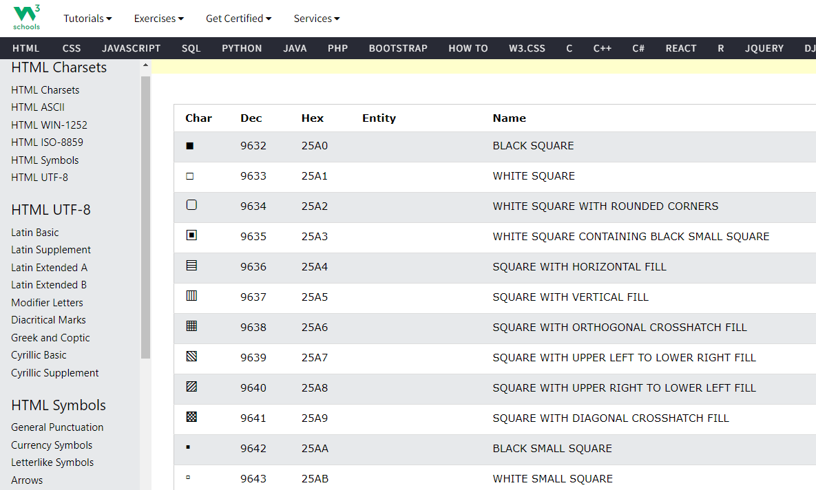
圖 2.1: w3schools的特殊符號
- 色彩置換,可以透過套件gt內的
info_paletteer查詢顏色的標籤。在R console執行
?gt::info_paletteer
查詢提供色板(palettes)的套件,如圖2.2:
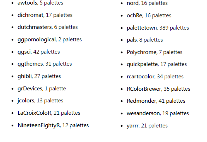
圖 2.2: 查詢色板(palettes)的套件名稱
圖2.2指出ggthemes提供31個提供色板(palettes)的物件,進一步查詢其內容,可在R console執行
gt::info_paletteer(color_pkgs ="ggthemes")
如圖2.3:
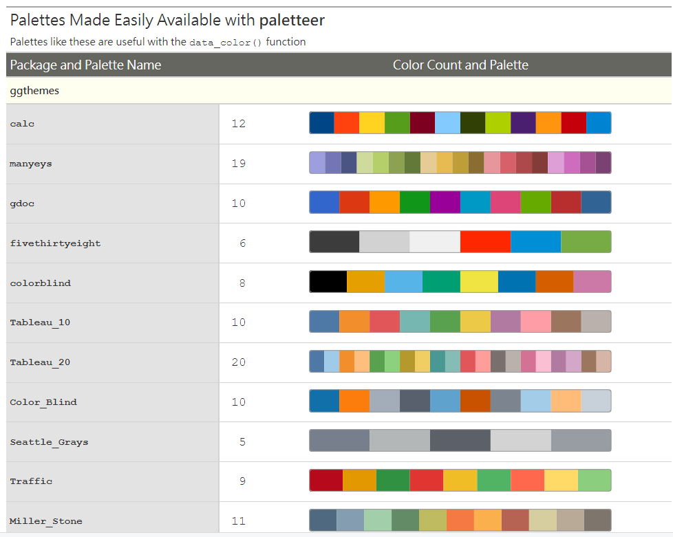
圖 2.3: 查詢ggthemes的色版物件
接下來要查詢顏色代號,以圖2.3為例,ggthemes內有一個物件calc,有12個顏色,查詢代號可以
paletteer::paletteer_d("ggthemes::calc")
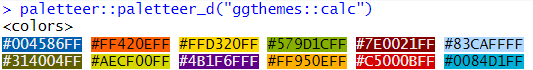
圖 2.4: 查詢ggthemes::calc 的顏色代號
找到自己喜歡的色彩與代碼,就可以用來填入表格內指定的項目:字形,符號,格子背景填滿等等。
2.3 套件 kableExtra 的表格製作
我們以前面表2.10使用的實質GDP資料 macro.csv
2.3.1 呈現簡單的 kable 表
load("data/macro.RData")
macro_tbl=data.frame(Country=rownames(macro),macro)
rownames(macro_tbl)=NULL
head(macro_tbl,10)
## Country rgdpe rgdpo cgdpe cgdpo
## 1 Argentina 1026128.1 1022513.25 1026128.1 1022513.25
## 2 Bulgaria 146484.2 139064.67 146484.2 139064.67
## 3 Brazil 2970570.8 2968825.50 2970570.8 2968825.50
## 4 Chile 428811.7 422309.03 428811.7 422309.03
## 5 China 19501140.0 19687162.00 19501140.0 19687162.00
## 6 Colombia 650044.0 656700.56 650044.0 656700.56
## 7 Costa Rica 93173.3 89731.84 93173.3 89731.84
## 8 Dominican Republic 170901.5 174065.56 170901.5 174065.56
## 9 Ecuador 191677.7 191572.67 191677.7 191572.67
## 10 Croatia 106672.8 106076.00 106672.8 106076.00接下來,kable內建產生的表格是LaTex Table。
library(kableExtra)
kbl_tbl1.tmp = kbl(head(macro_tbl,10), caption="")
kbl_tbl1 =kable_styling(kbl_tbl1.tmp, latex_options = "striped", full_width = F)
kbl_tbl1| Country | rgdpe | rgdpo | cgdpe | cgdpo |
|---|---|---|---|---|
| Argentina | 1026128.1 | 1022513.25 | 1026128.1 | 1022513.25 |
| Bulgaria | 146484.2 | 139064.67 | 146484.2 | 139064.67 |
| Brazil | 2970570.8 | 2968825.50 | 2970570.8 | 2968825.50 |
| Chile | 428811.7 | 422309.03 | 428811.7 | 422309.03 |
| China | 19501140.0 | 19687162.00 | 19501140.0 | 19687162.00 |
| Colombia | 650044.0 | 656700.56 | 650044.0 | 656700.56 |
| Costa Rica | 93173.3 | 89731.84 | 93173.3 | 89731.84 |
| Dominican Republic | 170901.5 | 174065.56 | 170901.5 | 174065.56 |
| Ecuador | 191677.7 | 191572.67 | 191677.7 | 191572.67 |
| Croatia | 106672.8 | 106076.00 | 106672.8 | 106076.00 |
表2.21的邏輯和gt一樣,先產生kable()LaTex Table物件,再用kable_styling美化 kbl_tbl1.tmp,程式內有幾項須要說明和注意的:
- 宣告
caption=""才會產生表格編號,如果須要對表格說明,在裡面打字即可,例如:。
caption="人口數據" kable_styling內的latex_options = "striped"會在表格列產生間錯的灰底,如果須要全白,將這個功能去除即可。在此,可以宣告字型大小,例如:font_size=10。更多的功能,請在R Console用?kable_styling查詢full_width = F如果宣告TRUE,表格會與頁面同寬。
2.3.2 在表底添加註釋與索引
在表底添加兩個註釋,可以使用函數footnote,但是,比gt簡單,可以一次就輸入兩條:
kbl_tbl1.tmp = kbl(head(macro_tbl,10), caption="")
kbl_tbl1 =kable_styling(kbl_tbl1.tmp, latex_options = "striped", full_width = F)
kbl_tbl2=footnote(kbl_tbl1,general_title = "",escape = TRUE,
         c("Source: 資料取自R 套件 pwt10.","Reference: Penn World Table, 10.01."))

kbl_tbl2| Country | rgdpe | rgdpo | cgdpe | cgdpo |
|---|---|---|---|---|
| Argentina | 1026128.1 | 1022513.25 | 1026128.1 | 1022513.25 |
| Bulgaria | 146484.2 | 139064.67 | 146484.2 | 139064.67 |
| Brazil | 2970570.8 | 2968825.50 | 2970570.8 | 2968825.50 |
| Chile | 428811.7 | 422309.03 | 428811.7 | 422309.03 |
| China | 19501140.0 | 19687162.00 | 19501140.0 | 19687162.00 |
| Colombia | 650044.0 | 656700.56 | 650044.0 | 656700.56 |
| Costa Rica | 93173.3 | 89731.84 | 93173.3 | 89731.84 |
| Dominican Republic | 170901.5 | 174065.56 | 170901.5 | 174065.56 |
| Ecuador | 191677.7 | 191572.67 | 191677.7 | 191572.67 |
| Croatia | 106672.8 | 106076.00 | 106672.8 | 106076.00 |
| Source: 資料取自R 套件 pwt10. | ||||
| Reference: Penn World Table, 10.01. |
另外,是對格子資訊標註,下表2.23對第一個變數坐上標 *;對China上標 a,然後製kable表,再用footnote說明
kbl_tbl2.tmp=macro_tbl
names(kbl_tbl2.tmp)[2]=paste0(names(kbl_tbl2.tmp)[2],footnote_marker_symbol(1))
kbl_tbl2.tmp[5,1]=paste0(kbl_tbl2.tmp[5,1],footnote_marker_alphabet(1))

kbl_tbl3.tmp=kbl(kbl_tbl2.tmp, align = "r", booktabs = T,escape = F,caption="")

kbl_tbl3=footnote(kbl_tbl3.tmp,
         symbol="Expenditure-side real GDP at chained PPPs (in million 2017 USD)",
         alphabet="中國大陸")

kable_styling(kbl_tbl3,full_width = F)| Country | rgdpe* | rgdpo | cgdpe | cgdpo |
|---|---|---|---|---|
| Argentina | 1026128.12 | 1022513.25 | 1026128.12 | 1022513.25 |
| Bulgaria | 146484.23 | 139064.67 | 146484.23 | 139064.67 |
| Brazil | 2970570.75 | 2968825.50 | 2970570.75 | 2968825.50 |
| Chile | 428811.66 | 422309.03 | 428811.66 | 422309.03 |
| Chinaa | 19501140.00 | 19687162.00 | 19501140.00 | 19687162.00 |
| Colombia | 650044.00 | 656700.56 | 650044.00 | 656700.56 |
| Costa Rica | 93173.30 | 89731.84 | 93173.30 | 89731.84 |
| Dominican Republic | 170901.52 | 174065.56 | 170901.52 | 174065.56 |
| Ecuador | 191677.72 | 191572.67 | 191677.72 | 191572.67 |
| Croatia | 106672.77 | 106076.00 | 106672.77 | 106076.00 |
| Indonesia | 2819440.75 | 2816072.25 | 2819440.75 | 2816072.25 |
| India | 8069977.50 | 8284343.00 | 8069977.50 | 8284343.00 |
| Sri Lanka | 259296.83 | 269025.34 | 259296.83 | 269025.34 |
| Mexico | 2405365.25 | 2363270.50 | 2405365.25 | 2363270.50 |
| Malaysia | 814839.25 | 751462.38 | 814839.25 | 751462.38 |
| Peru | 382137.50 | 375967.69 | 382137.50 | 375967.69 |
| Philippines | 805991.56 | 826499.00 | 805991.56 | 826499.00 |
| Poland | 1141621.00 | 1102457.25 | 1141621.00 | 1102457.25 |
| Romania | 509684.41 | 499683.66 | 509684.41 | 499683.66 |
| Russian Federation | 3907709.50 | 3899889.25 | 3907709.50 | 3899889.25 |
| Thailand | 1171981.62 | 1153407.62 | 1171981.62 | 1153407.62 |
| Turkey | 2106730.75 | 2158604.75 | 2106730.75 | 2158604.75 |
| Uruguay | 72320.16 | 70848.27 | 72320.16 | 70848.27 |
| South Africa | 738072.88 | 726021.00 | 738072.88 | 726021.00 |
| a 中國大陸 | ||||
| * Expenditure-side real GDP at chained PPPs (in million 2017 USD) |
以上兩個表格,將表底資訊分成兩塊,讀者有興趣可以是是看如何將兩種註腳合併。然後,此處小結是強調表格自動編號功能。和gt不同,gt只要有宣告物件即可。kable要編號的表格,則必須在程式區塊有kable()運算。所以,表2.21,表2.22和表2.23的程式區塊,都有重複執行kable()運算的一行,gt則不用這樣,但是要宣告tab_caption。如果沒有,表格會照樣產生,但是,不會有自動連續編號。
位了讓程式碼容易閱讀,我沒有採用 |> 這樣的功能6。用|>的寫法,請參考表2.24程式碼。
kbl_tbl2.tmp=macro_tbl
names(kbl_tbl2.tmp)[2]=paste0(names(kbl_tbl2.tmp)[2],footnote_marker_symbol(1))
kbl_tbl2.tmp[5,1]=paste0(kbl_tbl2.tmp[5,1],footnote_marker_alphabet(1))

kbl_tbl2.tmp |>

  kbl(align = "r", booktabs = T,escape = F,caption="") |>

  footnote(symbol="Expenditure-side real GDP at chained PPPs (in million 2017 USD)",
         alphabet="中國大陸") |>

kable_styling(full_width = F)| Country | rgdpe* | rgdpo | cgdpe | cgdpo |
|---|---|---|---|---|
| Argentina | 1026128.12 | 1022513.25 | 1026128.12 | 1022513.25 |
| Bulgaria | 146484.23 | 139064.67 | 146484.23 | 139064.67 |
| Brazil | 2970570.75 | 2968825.50 | 2970570.75 | 2968825.50 |
| Chile | 428811.66 | 422309.03 | 428811.66 | 422309.03 |
| Chinaa | 19501140.00 | 19687162.00 | 19501140.00 | 19687162.00 |
| Colombia | 650044.00 | 656700.56 | 650044.00 | 656700.56 |
| Costa Rica | 93173.30 | 89731.84 | 93173.30 | 89731.84 |
| Dominican Republic | 170901.52 | 174065.56 | 170901.52 | 174065.56 |
| Ecuador | 191677.72 | 191572.67 | 191677.72 | 191572.67 |
| Croatia | 106672.77 | 106076.00 | 106672.77 | 106076.00 |
| Indonesia | 2819440.75 | 2816072.25 | 2819440.75 | 2816072.25 |
| India | 8069977.50 | 8284343.00 | 8069977.50 | 8284343.00 |
| Sri Lanka | 259296.83 | 269025.34 | 259296.83 | 269025.34 |
| Mexico | 2405365.25 | 2363270.50 | 2405365.25 | 2363270.50 |
| Malaysia | 814839.25 | 751462.38 | 814839.25 | 751462.38 |
| Peru | 382137.50 | 375967.69 | 382137.50 | 375967.69 |
| Philippines | 805991.56 | 826499.00 | 805991.56 | 826499.00 |
| Poland | 1141621.00 | 1102457.25 | 1141621.00 | 1102457.25 |
| Romania | 509684.41 | 499683.66 | 509684.41 | 499683.66 |
| Russian Federation | 3907709.50 | 3899889.25 | 3907709.50 | 3899889.25 |
| Thailand | 1171981.62 | 1153407.62 | 1171981.62 | 1153407.62 |
| Turkey | 2106730.75 | 2158604.75 | 2106730.75 | 2158604.75 |
| Uruguay | 72320.16 | 70848.27 | 72320.16 | 70848.27 |
| South Africa | 738072.88 | 726021.00 | 738072.88 | 726021.00 |
| a 中國大陸 | ||||
| * Expenditure-side real GDP at chained PPPs (in million 2017 USD) |
承表2.20,下方的\(R^2\)只能用HTML呈現,對於習慣LaTex數字美感的人,會不太喜歡,套件kableExtra就可以保持這樣,如表2.25。
output=lm(wage~education+experience,data=dat)
Fstat=round(summary(output)$fstatistic[1],3)
table=papeR::prettify(summary(output),signif.stars=FALSE,digits=4)

table |>
  kable(align = "r", caption = '迴歸結果表', booktabs = TRUE) |>

  footnote(general_title = "",escape = TRUE,
           paste0("$F Stat$=",Fstat)
           ) |>

  footnote(general_title = "",escape = TRUE,
           paste0("$R^2$=",round(summary(output)$r.squared,3))
           ) |>

kable_styling(full_width = F)| Estimate | CI (lower) | CI (upper) | Std. Error | t value | Pr(>|t|) | |
|---|---|---|---|---|---|---|
| (Intercept) | -4.885 | -7.282 | -2.489 | 1.220 | -4.004 | < 0.001 |
| education | 0.9239 | 0.7638 | 1.084 | 0.08151 | 11.33 | < 0.001 |
| experience | 0.1058 | 0.07197 | 0.1397 | 0.01724 | 6.138 | < 0.001 |
| \(F Stat\)=66.948 | ||||||
| \(R^2\)=0.202 |
表2.25 的表底添加了兩個線性模型常用的配適統計量,請自我練習將F統計量的Pvalue黏貼於統計量之後,也就是如下表2.26
| Estimate | CI (lower) | CI (upper) | Std. Error | t value | Pr(>|t|) | |
|---|---|---|---|---|---|---|
| (Intercept) | -4.885 | -7.282 | -2.489 | 1.220 | -4.004 | < 0.001 |
| education | 0.9239 | 0.7638 | 1.084 | 0.08151 | 11.33 | < 0.001 |
| experience | 0.1058 | 0.07197 | 0.1397 | 0.01724 | 6.138 | < 0.001 |
| \(F Stat\)=66.948 (<0.000) | ||||||
| \(R^2\)=0.202 |
|>是Base R 的內建功能,意義和tidyverse的pipe一樣↩︎